We are all having to keep revising upwards our assessments of the mathematical capabilities of large language models. I have just made a fairly large revision as a result of ChatGPT 5.5 Pro, to which I am fortunate to have been given access, producing a piece of PhD-level research in an hour or so, with no serious mathematical input from me.
The background is that, as has been widely reported, LLMs are now capable of solving research-level problems, and have managed to solve several of the Erdős problems listed on Thomas Bloom’s wonderful website. Initially it was possible to laugh this off: many of the “solutions” consisted in the LLM noticing that the problem had an answer sitting there in the literature already, or could be very easily deduced from known results. But little by little the laughter has become quieter. The message I am getting from what other mathematicians more involved in this enterprise have been saying is that LLMs have got to the point where if a problem has an easy argument that for one reason or another human mathematicians have missed (that reason sometimes, but not always, being that the problem has not received all that much attention), then there is a good chance that the LLMs will spot it. Conversely, for problems where one’s initial reaction is to be impressed that an LLM has come up with a clever argument, it often turns out on closer inspection that there are precedents for those arguments, so it is still just about possible to comfort oneself that LLMs are merely putting together existing knowledge rather than having truly original ideas. How much of a comfort that is I will not discuss here, other than to note that quite a lot of perfectly good human mathematics consists in putting together existing knowledge and proof techniques.
I decided to try something a little bit different. At least in combinatorics, there are quite a lot of papers that investigate some relatively new combinatorial parameter that leads naturally to several questions. Because of the sheer number of questions one can ask, the authors of such papers will not necessarily have the time to spend a week or two thinking about each one, so there is a decent probability that at least some of them will not be all that hard. This makes such papers very valuable as sources of problems for mathematicians who are doing research for the first time and who will be hugely encouraged by solving a problem that was officially open. Or rather, it used to make them valuable in that way, but it looks as though the bar has just been raised. It is no longer enough that somebody asks a problem: it needs to be hard enough for an LLM not to be able to solve it.
In any case, a little over a week ago I decided to see how ChatGPT 5.5 Pro would fare with a selection of problems asked by Mel Nathanson in a paper entitled Diversity, Equity and Inclusion for Problems in Additive Number Theory. Nathanson has a remarkable record of being interested in problems and theorems that have later become extremely fashionable, which has led him to write a series of extremely well timed and therefore highly influential textbooks. In this paper, he argues for the interest of several other problems, some of which I will now briefly describe.
If  is a set of integers, then its sumset
  is defined to be
  . For a positive integer
  , the –fold sumset, denoted
  , is defined to be
  . Nathanson is interested in the possible sizes of given the size of . To that end one can define a set
  to be the set of all
  such that there exists a set with
  and
and  .
.
An obvious first question to ask is simply “What is ?” When  , the answer is the set of all integers between
  and
and  . It is an easy exercise to show that if , then
  , so this result is saying that all sizes in between can be realized. However, it is not true in general that can take every size between its minimum and maximum possibilities, and we do not currently have a complete description of .
Another natural question one can ask, and this is where ChatGPT came in, is how large a diameter you need if you want a set with and having prescribed sizes. (Of course, the size of must belong to .) Nathanson showed that for every ![t\in[2k-1,\binom{k+1}2]](https://s0.wp.com/latex.php?latex=t%5Cin%5B2k-1%2C%5Cbinom%7Bk%2B1%7D2%5D&bg=ffffff&fg=333333&s=0&c=20201002) there is a subset of
there is a subset of  with and
  , and asked whether the bound
  could be improved. ChatGPT 5.5 Pro thought for 17 minutes and 5 seconds before providing a construction that yielded a quadratic upper bound, which is clearly best possible. It wrote up its argument in a slightly rambling LLM-ish style, so I asked if it could write the argument up as a LaTeX file in the style of a typical mathematical preprint. After two minutes and 23 seconds it gave me that, after which I spent some time convincing myself that the argument was correct.
The basic idea behind both Nathanson’s argument and ChatGPT’s was that in order to obtain a set of a given size with a sumset of a given size, it is useful to build it out of a Sidon set, which means a set with sumset of maximal size (that is not quite the usual definition but it is the simplest to use in this discussion), and an arithmetic progression. Also, for a bit of fine tuning one can take an additional point near the arithmetic progression. Then if one plays around with the various parameters, one finds that one can obtain sets of all the sizes one wants. Nathanson doesn’t express his argument this way (it is Theorem 5 of this paper), instead giving an inductive argument, but I think, without having checked too carefully, that if one unravels his argument, one finds that effectively that is what he ends up with, and the Sidon set in question consists of powers of 2. ChatGPT obtained its improvement by simply using a more efficient Sidon set — it is well known that one can find Sidon sets of quadratic diameter. (One might ask why Nathanson didn’t do that in the first place: I think it is because the obvious idea of using a more efficient Sidon set becomes obvious only after one has redescribed his inductive construction. Is that what ChatGPT did? It is very hard to say.)
Next, I asked ChatGPT to see whether it could do the same for a closely related question, where instead of looking at the size of the sumset, one looks at the size of the restricted sumset, which is defined to be  . Unsurprisingly, it was able to do that with no trouble at all. I got it to write both results up in a single note, to avoid a certain amount of duplication. If you are curious, you can see the note here.
I then asked what it could do for general . I was much less optimistic that it would manage to do anything interesting, because the proof for makes fundamental use of the fact (due to Erdős and Szemerédi) that we know exactly which sizes we need to create. If we don’t know what the set is, then it seems that we are forced to start with a hypothetical set with and and build out of it a set of small diameter with the same property. As it happens, I still don’t know how to get round that difficulty (I’m mentioning that just to demonstrate that my mathematical input was zero, and I didn’t even do anything clever with the prompts), but Nathanson mentioned in his paper a remarkable paper of Isaac Rajagopal, a student at MIT, who must have got round the difficulty somehow, because he had managed to prove an exponential dependence of on  for each fixed .
I’ll leave the previous paragraph there, but Isaac has subsequently explained to me that that isn’t really the difficulty. His argument gives a complete description of when is sufficiently large, and if one wants to prove a polynomial dependence for fixed , then assuming that is sufficiently large is clearly permitted. The real difficulty is that constructing the sets with given sumset sizes was significantly more complicated, and necessarily so because the degree of the polynomial grows with , and one therefore needs more and more parameters to define the sets.
In any case, the task faced by ChatGPT was not to solve the problem from scratch, but to see whether it was possible to tighten up Isaac Rajagopal’s argument. Here’s what happened.
- After 16 minutes and 41 seconds, it came back with an argument that claimed to have improved the upper bound from exponential in to exponential in
 for any
  .
.
- I asked it to write that in preprint form too, which took it a further 47 minutes and 39 seconds.
- That preprint would have been hard for me to read, as that would have meant carefully reading Rajagopal’s paper first, but I sent it to Nathanson, who forwarded it to Rajagopal, who said he thought it looked correct.
- Both ChatGPT and Rajagopal speculated a little on what might need to be done to push things further and get a polynomial bound, so I got greedy and asked ChatGPT to give that a go.
- After 13 minutes and 33 seconds it told me it felt optimistic about the existence of such an argument but there were a couple of technical statements that needed checking.
- I asked it to check them.
- After 9 minutes and 12 seconds it got back to me with the check having been done, so I asked for this too to be written in preprint form.
- After 31 minutes and 40 seconds the “preprint” was ready. Here it is.
- Isaac Rajagopal looked at it and declared it to be almost certainly correct. It was clear that he meant this not just at a line-by-line level but at the level of ideas.
Isaac made some very interesting remarks about the nature of what the additional ideas were that ChatGPT contributed. Since, as I have already said, my mathematical input was zero, I invited him to write a guest section to this post. Just before we get to that, I want to raise a question (that will undoubtedly have been raised by others as well), which is simple: what should we do with this kind of content? Had the result been produced by a human mathematician, it would definitely have been publishable, so I think it would be wrong to describe it as AI slop. On the other hand, it seems pointless even to think about putting it in a journal, since it can be made freely available, and nobody needs “credit” for it (except that Isaac deserves plenty of credit for creating the framework on which ChatGPT could build). I understand that arXiv has a policy against accepting AI-written content, which makes good sense to me. So maybe there should be a different repository where AI-produced results can live. But various decisions would need to be made about how it was organized. I myself think that one would probably want to have some kind of moderation process, so that results would be included only if a human mathematician was prepared to certify that they were correct — or, better still, that they had been formalized by a proof assistant — and perhaps also that they answered a question that had been asked in a human-written paper. On the other hand, I wouldn’t want a moderation process that created vast amounts of work (unless the work was itself done by AI, but there are obvious dangers in going down that route). Anyway, until these questions are answered, this result is available from the link above, and perhaps, now that LLMs are so good at literature search, that will be enough to make it findable by anyone who wants to know whether Nathanson’s problem has been solved.
Isaac’s evaluation of what ChatGPT achieved
With just a few prompts, ChatGPT was able to improve the upper bound on  (which I will define very soon) from exponential in to polynomial in . While its first improvement of the bound, from exponential in to exponential in
  , was a routine modification of my work, the improvement to polynomial in is quite impressive. To do this, ChatGPT came up with an idea which is original and clever. It is the sort of idea I would be very proud to come up with after a week or two of pondering, and it took ChatGPT less than an hour to find and prove, using similar methods to those in my own proof. My goal is to explain that idea, in a manner that will be digestible to my friends who are computer science majors as well as my math major friends.
The problem of bounding is closely related to a problem I worked on at the Duluth REU (Research Experience for Undergrads) program, of determining  . In particular, is the set of possible -fold sumset sizes
  , where can be chosen to be any set of integers. is the minimal
  such that we can achieve all of the values of using -element sets
  . I spent last summer explicitly characterizing the set for large , by constructing sets such that achieves all sizes which I could not rule out as impossible. So, can be upper-bounded by optimizing my constructions.
I constructed these sets by combining smaller component sets which are simpler to analyze. Some of these components are the geometric series

for various values of  and
and  . Unfortunately, the elements of
  and
and  are exponentially large in terms of . So, I asked ChatGPT (through Tim) whether there exist sets of
  elements which have similar sumset sizes to these geometric series, but contain only numbers of polynomial size in : I had no idea if this was possible, or how to begin constructing such sets. ChatGPT came back with an answer, constructing sets
  and
and  which behave like “half a geometric series squeezed into a polynomial interval,” which is counterintuitive. Before I discuss the construction of and , I will explain the important properties of the sumset sizes of and which they recreate.
For  , a set is called a
  set if the only solutions to

with  in are the “trivial” solutions, by which I mean that one side of the equation is a reordering of the other side. If is a set of size , then elements of correspond exactly to choices of elements of , with repetition allowed. Using “stars and bars,” one can see that
  and this is the maximum possible value of among sets of size . So, another definition is that is a set if
  . Sidon sets, which Tim discussed, are exactly
  sets.
sets.
To make things more concrete, let us assume that  in (1). Then, is a
  set, but it is not a
  set because of the relations

for any choice of  in
in  . In particular,
  , as these
  relations are the only ones preventing from being a set. lacks the relations in (2) because
  is not in . So, is a set, but it is not a
  set because of the relations

for any choices of  in
in  . This gives
  relations, and one can check that
  . To summarize, we have seen that
(a) is a  set.
set.
(b)  is a linear function of .
(c) is a  set.
set.
(d)  is a quadratic function of .
ChatGPT was able to find sets and of elements which satisfy (a)-(d), but whose elements all have polynomial size in . The construction of and uses  -dissociated sets, which are sets where the only solutions to

with  and in are the “trivial” solutions, i.e.
  and one side of the equation is a reordering of the other side. For
  , it is possible to construct an -dissociated set
  , where is approximately
  , and in particular polynomial in
  . Constructions of such a
  using finite fields date back to Singer (1938) and Bose–Chowla (1963) and are described in Appendix 1. Define

and

In hindsight, I have good intuition for the construction of and . All of the relations in (2) and (3) are formed by combining one or two relations of the form  . There are approximately relations of the form
  in and , and approximately
  such relations in and . There are few other low-order relations in and , and similarly in and because is -dissociated. So, and manage to contain half as many -relations as their geometric series counterparts, while also containing few low-order relations.
We now see why (a)-(d) hold with and replaced by and , respectively. For concreteness, we assume that and  , so contains no nontrivial relations as in (4) with
  . Then, is a set, but it is not a set because of the relations

for any choice of  in
in  . If we let
  , we can check that
  is linear in . In particular, (a) and (b) hold with replaced by , and the linear function replaced by
  . We can also see that is a set, but it is not a set because of the relations

for any  in . If we let
  , we can check that
  is quadratic in . In a similar manner, (c) and (d) hold with replaced by , and the quadratic function replaced by
  .
.
Even though I can motivate it in retrospect, ChatGPT’s idea to use -dissociated sets to control relations of order at most feels quite ingenious. As far as I can tell, this idea is completely original.
ChatGPT’s proof that its construction produces the desired values of is very similar to my proof that the sets which I construct achieve all possible values of , after replacing and by and , respectively. Properties (a)-(d) capture many of the important properties of and (or and ) which are used in this proof. The final constructions involve combining the sets and (or and in my paper) for each value of  between
  and with another set which is the union of an arithmetic progression and a point. Intuitively, and (or and ) have large sumsets, while arithmetic progressions have small sumsets, so it is plausible that one could get sets which achieve all the medium-sized sumsets by combining them. However, the proof of this is quite involved, and it occupies Section 4 of my paper and the entirety of the ChatGPT preprint. In Appendix 2, I work out the details of the ChatGPT construction to show that for sufficiently large,

For comparison, it is easy to see that is at least on the order of  , and it is unknown what the real value is. In Appendix 3, I give details of the correspondence between my paper and the ChatGPT preprint, which will be helpful for those who want to read either.
Finally, I want to express my deep gratitude to Tim for allowing me to contribute to this blog. I am still stunned by the coincidence that the problem he chose to put into ChatGPT 5.5 Pro led him to my paper on the arXiv.
Tim on what this means for mathematical research
I would judge the level of the result that ChatGPT found in under two hours to be that of a perfectly reasonable chapter in a combinatorics PhD. It wouldn’t be considered an amazing result, since it leant very heavily on Isaac’s ideas, but it was definitely a non-trivial extension of those ideas, and for a PhD student to find that extension it would be necessary to invest quite a bit of time digesting Isaac’s paper, looking for places where it might not be optimal, familiarizing oneself with various algebraic techniques that he used, and so on.
It seems to me that training beginning PhD students to do research, which has always been hard (unless one is lucky enough, as I have often been, to have a student who just seems to get it and therefore doesn’t need in any sense to be trained), has just got harder, since one obvious way to help somebody get started is to give them a problem that looks as though it might be a relatively gentle one. If LLMs are at the point where they can solve “gentle problems”, then that is no longer an option. The lower bound for contributing to mathematics will now be to prove something that LLMs can’t prove, rather than simply to prove something that nobody has proved up to now and that at least somebody finds interesting.
I would qualify that statement in two ways though. First, there is the obvious point that a beginning PhD student has the option of using LLMs. So the task is potentially easier than proving something that LLMs can’t prove: it is proving something in collaboration with LLMs that LLMs cannot manage on their own. I have done quite a lot of such collaboration recently and found that LLMs have made useful contributions without (yet) having game-changing ideas.
A second point is that I don’t know how much of what I have said generalizes to other areas of mathematics. Combinatorics tends to be quite focused on problems: you start with a question and you reason back from the question or if you reason forwards you do so very much with the question in mind. In other areas there can be much more of an emphasis on forwards reasoning: you start with a circle of ideas and see where it leads. To do it successfully, you need to have some way of discriminating between interesting observations and uninteresting ones, and it isn’t obvious to me what LLMs would be like at that.
Of course, everything I am saying concerns LLMs as they are right now. But they are developing so fast that it seems almost certain that my comments will go out of date in a matter of months. It is also almost certain that these developments will have a profoundly disruptive effect on how we go about mathematical research, and especially on how we introduce newcomers to it. Somebody starting a PhD next academic year will be finishing it in 2029 at the earliest, and my guess is that by then what it means to undertake research in mathematics will have changed out of all recognition.
I sometimes get emails from people who are interested in doing mathematical research but are not sure whether that makes sense any more as an aspiration. I have a view on that question, but it may very well change in response to further developments. That view is that there is still a great deal of value in struggling with a mathematics problem, but that the era where you could enjoy the thrill of having your name forever associated with a particular theorem or definition may well be close to its end. So if your aim in doing mathematics is to achieve some kind of immortality, so to speak, then you should understand that that won’t necessarily be possible for much longer — not just for you, but for anybody. Here’s a thought experiment: suppose that a mathematician solved a major problem by having a long exchange with an LLM in which the mathematician played a useful guiding role but the LLM did all the technical work and had the main ideas. Would we regard that as a major achievement of the mathematician? I don’t think we would.
So what is the point of struggling with a difficult mathematics problem? One answer is that it can be very satisfying to solve a problem even if the answer is already known, but I don’t think that is a sufficient reason to spend several years of your life on this peculiar activity. A better answer is that by solving hard problems you get an insight into the problem-solving process itself, at least in your area of expertise, in a way that you simply don’t if all you do is read other people’s solutions. One consequence of this is that people who have themselves solved difficult problems are likely to be significantly better at using solving problems with the help of AI, just as very good coders are better at vibe coding than not such good coders, or people who have a solid grasp of how to do basic arithmetic are likely to be more skilled at using calculators (and especially at noticing when an answer feels off). Mathematics is a highly transferable skill, and that applies to research-level mathematics as well. By doing research in mathematics, you may not get the same rewards as your equivalents a generation ago, but there is a good chance that you will be equipping yourself very well for the world we are about to experience.
Appendix 1 (Isaac)
We will construct an -dissociated set , where is approximately  . This construction is a very minor modification of Bose–Chowla (1963)’s construction of a set, which I learned about from this paper. For whatever reason, the GPT preprint (Lemma 3.1) uses a different, less efficient construction using moment curves.
Let  be a prime, let
  , let
, let  be the finite field with
  elements and fix a generator
  of
of  , so that is equal to
  . Define a set of
  elements

Then, each element  corresponds to a unique value of
  , by taking
  . Now an additive relation of the form in (4) with
  can be reframed by taking powers of as

As is a degree- extension of
  and is a generator of as an -extension, this means that does not satisfy any nonzero polynomials in
 ![\mathbb{F}\sb{p}[x]](https://s0.wp.com/latex.php?latex=%5Cmathbb%7BF%7D%5Csb%7Bp%7D%5Bx%5D&bg=ffffff&fg=333333&s=0&c=20201002) of degree
of degree  . So, both sides of (6) are identical as polynomials in
 ![\mathbb{F}_{p}[\theta]](https://s0.wp.com/latex.php?latex=%5Cmathbb%7BF%7D_%7Bp%7D%5B%5Ctheta%5D&bg=ffffff&fg=333333&s=0&c=20201002) and thus the additive relation in (4) is trivial. So, is -dissociated, and of course one can prune a few elements to reduce to size .
and thus the additive relation in (4) is trivial. So, is -dissociated, and of course one can prune a few elements to reduce to size .
Appendix 2 (Isaac)
Fix constants  such that
  (in my paper I arbitrarily chose
  ). Let the two sets in (5) be called
  and
and  . Let
. Let ![[a,b]](https://s0.wp.com/latex.php?latex=%5Ba%2Cb%5D&bg=ffffff&fg=333333&s=0&c=20201002) denote the set of integers
denote the set of integers  satisfying
  . Similarly to my paper, the constructions of such that achieves the desired sizes will combine sets of the following four types:
![B_{j,b} := [0,b-2] \cup \{b-2+j\}](https://s0.wp.com/latex.php?latex=B_%7Bj%2Cb%7D+%3A%3D+%5B0%2Cb-2%5D+%5Ccup+%5C%7Bb-2%2Bj%5C%7D&bg=ffffff&fg=333333&s=0&c=20201002) with choices of
with choices of ![b \in [3, k-k^\gamma]](https://s0.wp.com/latex.php?latex=b+%5Cin+%5B3%2C+k-k%5E%5Cgamma%5D&bg=ffffff&fg=333333&s=0&c=20201002) and
and ![j \in [1,hb]](https://s0.wp.com/latex.php?latex=j+%5Cin+%5B1%2Chb%5D&bg=ffffff&fg=333333&s=0&c=20201002) .
. for each value of
 ![m \in [3, h]](https://s0.wp.com/latex.php?latex=m+%5Cin+%5B3%2C+h%5D&bg=ffffff&fg=333333&s=0&c=20201002) , with choices of
, with choices of ![r_m \in [0, (k-b)^\alpha]](https://s0.wp.com/latex.php?latex=r_m+%5Cin+%5B0%2C+%28k-b%29%5E%5Calpha%5D&bg=ffffff&fg=333333&s=0&c=20201002) .
. for each value of
 ![m \in [2,h-1]](https://s0.wp.com/latex.php?latex=m+%5Cin+%5B2%2Ch-1%5D&bg=ffffff&fg=333333&s=0&c=20201002) , with choices of
, with choices of ![u_m \in [0, (k-b)^\beta]](https://s0.wp.com/latex.php?latex=u_m+%5Cin+%5B0%2C+%28k-b%29%5E%5Cbeta%5D&bg=ffffff&fg=333333&s=0&c=20201002) .
.- A set of the correct size so that
 .
.
One reason that this construction needs to be complicated is that we need to create at least  many sets. To do this, we vary
  parameters
  and
and  in the domain
 ![[0,k^\alpha]](https://s0.wp.com/latex.php?latex=%5B0%2Ck%5E%5Calpha%5D&bg=ffffff&fg=333333&s=0&c=20201002) and parameters
and parameters  and
and  in the domain
 ![[1,hk]](https://s0.wp.com/latex.php?latex=%5B1%2Chk%5D&bg=ffffff&fg=333333&s=0&c=20201002) . We can choose
. We can choose  to be slightly bigger than
  , and then the above construction gives us
  different sets where
  can be made arbitrarily small. So, if we were to remove any of the above parameters from the construction, and not change the others, this construction would no longer create many sets. In comparison, Nathanson’s construction when only needs to create
  sets. He does this by combining a Sidon set, an arithmetic progression, and one extra value, and varying the size of the arithmetic progression and the extra value in ranges of size
  .
.
We want to combine  sets
sets  , which are given by
  , for the
  values of
 ![m \in [3,h]](https://s0.wp.com/latex.php?latex=m+%5Cin+%5B3%2Ch%5D&bg=ffffff&fg=333333&s=0&c=20201002) , for the values of , and a set. By Appendix 1, for all
, for the values of , and a set. By Appendix 1, for all  , there exists a -dissociated set
  of diameter
  . By the constructions of and , we can take each
 ![A_i \subseteq [0,M]](https://s0.wp.com/latex.php?latex=A_i+%5Csubseteq+%5B0%2CM%5D&bg=ffffff&fg=333333&s=0&c=20201002) , where
, where  . Let
. Let  have basis vectors
  . To combine , we can define
  as
as

Similarly to my Lemma 4.9, this construction ensures that the generating function product  holds, which is the identity that both my paper and the GPT preprint use (see either paper for a definition of these generating functions). By (the standard) Lemma 2.3 of the GPT preprint, is Freiman-isomorphic of order to a subset of
 ![[0,2qM(2hM)^{2q-1}]](https://s0.wp.com/latex.php?latex=%5B0%2C2qM%282hM%29%5E%7B2q-1%7D%5D&bg=ffffff&fg=333333&s=0&c=20201002) . Therefore, for sufficiently large (the whole construction relies on this for the same reasons as in my paper),
. Therefore, for sufficiently large (the whole construction relies on this for the same reasons as in my paper),

Appendix 3 (Isaac)
In Section 4.2 of my paper, I use a different, simpler construction to construct sets achieving the values in which have  , for some small
  . These sets are subsets of
  , meaning that all elements have polynomial size in . This is observed in Section 5 of the GPT preprint.
Section 4.3 of my paper carries out the construction which combines many components including and . This corresponds to Sections 2, 3, 4, and 6 of the GPT preprint. This section has a lot of moving parts; I give an outline in Section 4.3.1.
In Section 4.3.2, I describe how the different components will be combined, using a construction which I call the disjoint union, and introduce generating functions  as a bookkeeping tool to keep track of the sumset sizes of a set . This corresponds to Section 2 and Section 4 of the GPT preprint.
In Section 4.3.3, I compute the generating function of each of the component sets, including  (Lemma 4.15) and
  (Lemma 4.17). This corresponds to Section 3 and Section 6.1 of the GPT preprint. In particular,
  is computed in Lemma 3.3 and
  is computed in Lemma 3.4. Once these generating functions have been computed, the remainder of the proof is almost identical in my paper and in the GPT preprint.
In Section 4.3.4, I put all the pieces together to show that as we range over the sets which I have constructed, the values of will assume all of the elements of  . The key idea is to show that the set of all values of forms an interval, and contains numbers both smaller than
  and equal to
  .
.


 be a polynomial map in
  complex variables, whose Jacobian
  is a non-zero constant. Then
  is invertible (with polynomial inverse).
  which has non-zero constant Jacobian, but is not invertible.


 , so the fact that all non-constant coefficients of this polynomial vanish looks like a massive cancellation involving
  equations, which is much larger than the
  degrees of freedom for a generic degree seven polynomial map of three variables. So finding such a polynomial looks highly unlikely to be located by brute force.
 to an equivalent affine variety. Namely, we will show
 that is isomorphic to
  which is locally injective, but not globally injective.
  and using the previously mentioned fact that local injectivity implies non-zero constant Jacobian. Our objective is now to find data
  ,
,  . But the equivalence between
  ), so we do not highlight this aspect of the construction.)
 of linear homogeneous polynomials
  of two complex variables
  .
.  of quadratic homogeneous polynomials
  of two complex variables
  of two complex variables
  here refers to the
 respectively. Furthermore, we have a multiplication map
  , mapping a pair
  of a linear polynomial
  and a quadratic polynomial
  to a cubic polynomial
 to
to  , is clearly polynomial; it is given explicitly in coordinates as
 for some non-zero complex numbers
  , then the product
  is scaled by
  :
:  .
.  for some invertible linear transformation
  , then the product
  :
:  .
.
 .
.
 is of course larger than the four-dimensional range
 modify the linear and quadratic polynomials
  but not their product
  . But even if one quotients out by this symmetry
  will split into the product
  of three independent linear polynomials. Then there are three pairs

 to obtain a useful normalization. If
  is a linear polynomial and
  is a quadratic polynomial, the
  can be defined by the determinant


 -invariant: for any
  , we have
 (which translate the roots
  by
by  while leaving
  unchanged) and for inversions
  (which map
  while mapping
  and
and  respectively), and then noting that these transformations generate all of
  . They also interact very nicely with scaling:
 :
: 


 . As the resultant is non-vanishing, the root
  of
of  of
of  ), thus
  for some complex number
  and
and  for some complex numbers
  , with the resultant condition
  (so in particular
  are also non-zero). It is then clear that if one perturbs
  ), then the root
  of
of  ), while the roots
  of
of  , one can reconstruct which of the three roots of this cubic polynomial will be the perturbed root of
  of
of 

 in two variables. Indeed, every such operator
  generates an affine hyperplane
  that avoids the origin, and conversely by duality every affine hyperplane avoiding the origin arises in this form uniquely. Just as the cubic polynomials in
  can also be factored into three linear differential operators, e.g.,
 is non-zero. The
  around the Riemann sphere by Möbius transformations. As these transformations are
  -transitive, the actual selection of such roots is not too important (and the scaling symmetry similarly makes the choice of leading coefficient
  for independent first-order operators
  .
.  for independent first-order operators
  .
.  for some first-order operator
  .
.
 , thus
  with
with  . Using
 is non-zero, then the second equation
  can be solved for
  ,
, 
 can be solved for
  ,
, 
 is uniquely determined by
  by a change of variables which is Laurent in
  . Thus we have a nice birational equivalence

 of
of 
 by polynomial changes of variable, since we can reconstruct
  from the coordinates
 is just
 have a unique affine solution
  (as opposed to the six possible solutions that Bezout’s theorem might suggest – the other five solutions live on the line at infinity). So the fiber here is also affine:
 , which is already extremely close to being isomorphic to the affine space
  , and that a global polynomial coordinate chart for
  and
and  fibers can be constructed.
 to denote any multiple of
  . Thus, for instance, the equation
  implies that


 , which on substitution into
  ; substituting this back into either
  .
.
 into
into 
 more explicitly as
  , then we have


 error term in
  , and doing a little more algebra, we thus have a polynomial change of variables


 . This already gives (a) and thus completes the proof of Theorem

 to the
  coefficients of
  coefficient which is constrained to equal
  ), we obtain a polynomial map

 . This is essentially the original example up to trivial changes of variable; indeed, one can check that the map
 fit together into a ring — let’s call it R — and
  is an R-module, which you’re gonna hope to show is more or less finitely generated by doing some homological algebra in the category of R-modules. This really goes all the way back to my original paper with Venkatesh and Westerland, which treats a special case of this. Anyway, a key point in this paper with Mark is that life is really good if R is actually finite-dimensional over k, which doesn’t happen in the Hurwitz space cases we used to exclusively think about. In cases like this, it turns out that
  vanishes in some range i < cn + d.
 with all j < i, not just j=0 as in our paper. But what that allows him to do is argue that if, for some c,d it is true that
  is easily checked to be
  . However, the map
  ,
,  and
and  are homogeneous with respect to the grading where
  ,
,  and
and  ; their degrees are
  ,
,  and
and  . I’m not sure what to make of this, but it surely matters.
 , you get a cubic relation in the remaining variable. Here they are
 cubic. Then the discriminants of the three cubics are
  ,
,  ,
,  where
where  have no common zeroes. Roughly speaking, our map should have special behavior over the loci
  ,
,  ,
,  and
and  . The fact that $p$, $q$ and $r$ each appear cubed means that the variables
  and
and  should have three fold branching over the loci
 and magnetic permeability
  of the vacuum, whose product is
  . This is convenient but not necessary, as explained here:
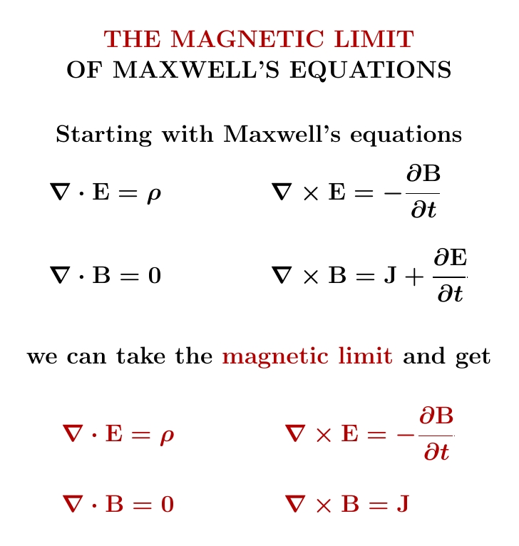
 is zero, since this is typically close to true in a plasma. However Heras does not do this, nor does the original paper:
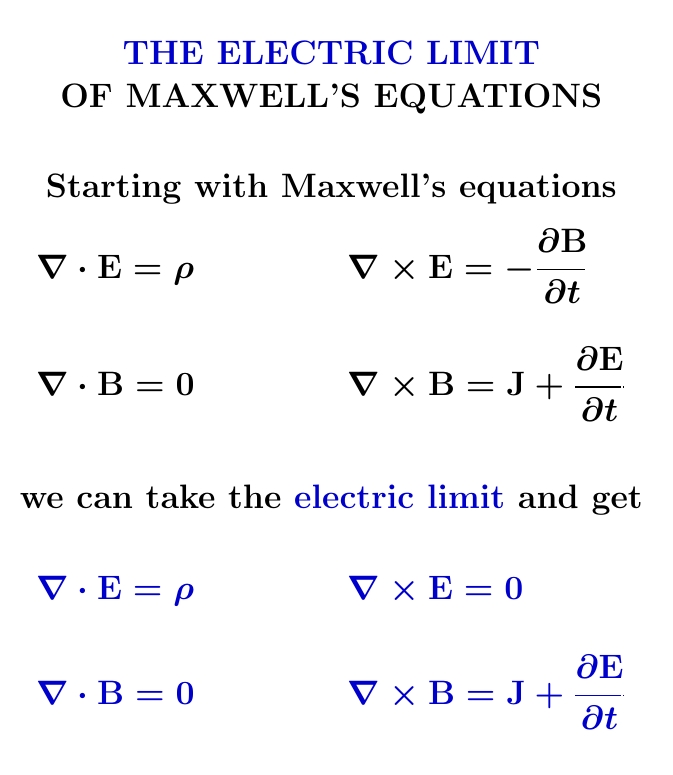
 .
. .
.
 for the space of column vectors with two bioctonion entries.
![[x,y,z]=\frac{1}{2}(x(y^{\dagger}z)+z(y^{\dagger}x))](https://s0.wp.com/latex.php?latex=%5Bx%2Cy%2Cz%5D%3D%5Cfrac%7B1%7D%7B2%7D%28x%28y%5E%7B%5Cdagger%7Dz%29%2Bz%28y%5E%7B%5Cdagger%7Dx%29%29+&bg=ffffff&fg=333333&s=0&c=20201002)
 -graded real Lie algebra
 The Lie algebra
  consists of all linear maps from
  to itself that are of this form:
![x \mapsto [a,b,x] - [b,a,x]](https://s0.wp.com/latex.php?latex=x+%5Cmapsto+%5Ba%2Cb%2Cx%5D+-+%5Bb%2Ca%2Cx%5D+&bg=ffffff&fg=333333&s=0&c=20201002)
 These maps are called real inner derivations. They form a Lie algebra since the commutator of two such maps is another such map. With a bit more work we can define other operations making all of
  into a
  and a Lie subalgebra
  whose Lie algebra is
 is a nice kind of manifold called a
  Our original Jordan triple,
  is then the tangent space of that point! So,
  :
:![\mathfrak{e}_6 = \big[\mathfrak{so}(10) \textstyle{\oplus} \mathfrak{u}(1)\big] \textstyle{\oplus} \mathbb{O}_\mathbb{C}^2](https://s0.wp.com/latex.php?latex=%5Cmathfrak%7Be%7D_6+%3D+%5Cbig%5B%5Cmathfrak%7Bso%7D%2810%29+%5Ctextstyle%7B%5Coplus%7D+%5Cmathfrak%7Bu%7D%281%29%5Cbig%5D+%5Ctextstyle%7B%5Coplus%7D+%5Cmathbb%7BO%7D_%5Cmathbb%7BC%7D%5E2+&bg=ffffff&fg=333333&s=0&c=20201002)
 The even part of our 3-graded Lie algebra,
  generates the stabilizer of a point in the bioctonionic plane. The odd part, our friend
  is the tangent space of that point.
 while the odd part itself transforms as the 16-dimensional complex spinor representation of
  Ignoring the extra
  for a moment, this is exactly what we see in a
  grand unified theory: gauge bosons in the adjoint representation, and one generation of fermions in the 16-dimensional spinor representation.
 In a Jordan triple
  their role is played by tripotents: elements
  with
with![[e,e,e] = e](https://s0.wp.com/latex.php?latex=%5Be%2Ce%2Ce%5D+%3D+e+&bg=ffffff&fg=333333&s=0&c=20201002)
![w \mapsto [e,e,w]](https://s0.wp.com/latex.php?latex=w+%5Cmapsto+%5Be%2Ce%2Cw%5D&bg=ffffff&fg=333333&s=0&c=20201002) has eigenvalues 0, 1/2, and 1, so
has eigenvalues 0, 1/2, and 1, so 
 A tripotent is called minimal when its Peirce 1-space is one-dimensional. Two tripotents
  are called colinear when each lies in the other’s Peirce 1/2-space.
![[-,-,-]](https://s0.wp.com/latex.php?latex=%5B-%2C-%2C-%5D&bg=ffffff&fg=333333&s=0&c=20201002) is linear in the first and last slot, but conjugate-linear in the middle slot. So, if you multiply a tripotent by a phase
is linear in the first and last slot, but conjugate-linear in the middle slot. So, if you multiply a tripotent by a phase  you get a new tripotent:
![[\alpha e, \alpha e, \alpha e] = \alpha \overline{\alpha} \alpha e = \alpha e](https://s0.wp.com/latex.php?latex=%5B%5Calpha+e%2C+%5Calpha+e%2C+%5Calpha+e%5D+%3D+%5Calpha+%5Coverline%7B%5Calpha%7D+%5Calpha+e+%3D+%5Calpha+e&bg=ffffff&fg=333333&s=0&c=20201002)
 (even part in brackets)
![\mathfrak{e}_6 = [\mathfrak{so}(10) \oplus \mathfrak{u}(1)] \oplus \mathbb{O}_\mathbb{C}^2](https://s0.wp.com/latex.php?latex=%5Cmathfrak%7Be%7D_6+%3D+%5B%5Cmathfrak%7Bso%7D%2810%29+%5Coplus+%5Cmathfrak%7Bu%7D%281%29%5D+%5Coplus+%5Cmathbb%7BO%7D_%5Cmathbb%7BC%7D%5E2&bg=ffffff&fg=333333&s=0&c=20201002)

![\mathfrak{so}(10) = [\mathfrak{su}(5) \oplus \mathfrak{u}(1)] \oplus \mathfrak{a}_5(\mathbb{C})](https://s0.wp.com/latex.php?latex=%5Cmathfrak%7Bso%7D%2810%29+%3D+%5B%5Cmathfrak%7Bsu%7D%285%29+%5Coplus+%5Cmathfrak%7Bu%7D%281%29%5D+%5Coplus+%5Cmathfrak%7Ba%7D_5%28%5Cmathbb%7BC%7D%29&bg=ffffff&fg=333333&s=0&c=20201002)

![\mathfrak{su}(5) = [\mathfrak{g}_{\mathrm{SM}}] \oplus \mathrm{M}_{3,2}(\mathbb{C})](https://s0.wp.com/latex.php?latex=%5Cmathfrak%7Bsu%7D%285%29+%3D+%5B%5Cmathfrak%7Bg%7D_%7B%5Cmathrm%7BSM%7D%7D%5D+%5Coplus+%5Cmathrm%7BM%7D_%7B3%2C2%7D%28%5Cmathbb%7BC%7D%29&bg=ffffff&fg=333333&s=0&c=20201002)
 is the Jordan triple of antisymmetric
  complex matrices,
  is the Jordan triple of
  complex matrices,
  and
and
 Descend the table twice:
 which has real inner automorphism group
 Its Peirce
  latex W’ = \mathfrak{a}_5(\mathbb{C}),$ with real inner automorphism group
 (colinear with
  so living in
  ). Its Peirce
  latex W’$ is
  with real inner automorphism group exactly
 and
and  sits inside the original group
  At each we step take the subgroup that acts with determinant
  and preserves the chosen tripotent up to a phase; this gives a chain of subgroups whose members are
  and
and  so we get the embeddings
 grand unified theory down to the Standard Model. And it’s well known that restricting the 16-dimensional complex spinor representation of
  along this chain gives precisely the Standard Model representation
  on one generation of fermions! So we get one generation of Standard Model fermions this way.
 we have projections
  and
and  onto its three eigenspaces: its so-called Peirce projectors. Since we get the Standard Model structure using two minimal tripotents
  , there are nine composites of two Peirce projectors we can apply to this triple. This is how we pick out the different kinds of fermions!

 Six irreducible pieces, six particle types.
 Those six match up one-to-one with the particle types:


 1, +1/3)


 and
and  —all vanish, which is why we land on six pieces and not nine.
 the representation
  and even the split of one generation into its six particle multiplets as distinct Peirce components—all comes out of the single object
  you get the same result by choosing three mutually colinear tripotents instead of two—but for that, read our paper!
.")


 , the
, the  is a random natural number with distribution
 divides
  . However, the new observation is that these random variables
 , and one variable at the primes
  . At a given choice of
  ,
,  , leading to
  in this case. Additional visualizations in the app display the distribution of each
  , which among other things can be used to give a quick solution to


 relating to the Gilbreath conjecture, which I will call the “Gilbreath expectation sequence” here for lack of a better name. The definition of the sequence is as follows. Consider a “Gilbreath array” which is an inverted pyramid, where the top entries are
  independent exponential random variables of mean 1, and all the other entries are the absolute values of the differences of the two entries immediately above it. Thanks to the
  ):
):
 are defined to be the expectation of these values. (The process is stationary, so in fact any entry on the
  row will have expectation
  .)
.)  normalized prime gaps (which have expectation about
  , and are conjecturally distributed asymptotically according to a geometric distribution), then standard conjectures (e.g., the prime tuples conjecture) predict that the
  row entries should decay like
  , at least for small
  . So the Gilbreath conjecture appears to be tied to how fast the sequence
  decays with
  (the orange line in the above figure); for the remaining
  Gilbreath arrays to obtain a numerical approximation (in blue), which (as per the law of large numbers) agreed well with the theoretical values. A
  , maintaining the good fit:
 .
.
 and
and  (empirically
  ), where
  is the number of 1’s in the binary expansion of
  that is intended to explain much of the non-monotonic behavior of

 version of this picture looks like (with the spike positioned at the 32th entry):
 (if we index the rows starting from zero), which is at least of the same shape as the empirical prediction, albeit with different constants. (This sequence is also known as


 , consisting of
  self-adjoint complex matrices. Similarly, the algebra of observables of an qutrit is the Jordan algebra
  , consisting of
  self-adjoint complex matrices.
 with
with 
 , consisting of
  is not a Jordan algebra when
  is bigger than 3.
 , in fact a certain subgroup of this acts trivially on all known particles. If we mod out by that, we’re left with a group called
  , which is
 —so that’s what I mean by the symmetries of an octonionic qutrit.
 are Jordan subalgebras of

 is the stabilizer of
  —that is, the subgroup of
  is the identity component of the stabilizer of
  .
. , while
  also contains those symmetries that are described by antiunitary operators. The CPT symmetry of the Standard Model is antiunitary, for example.
 are Jordan subalgebras of

 -invariant operations on
  . We then use this description to reprove Todorov and Dubois–Violette’s special case of Theorem 2. Then we show that
  . This lets us prove that
  with
with  ,
,  and
and  . Theorem 2 then follows from Todorov and Dubois-Violette’s special case. We conclude by using these results to prove Theorem 1.
 show up from the relation between octonionic qutrits, complex qutrits and complex qubits. You’ll see that in the proof of Lemma 4.
 or
or  sitting inside
  , where
  is some normed division algebra contained in a bigger normed division algebra
  .
.
 Taking logs we see

 This constant is called the
  which is defined by


 is the
  is the Riemann zeta function. By the way, this formula shows that calling
  a fancier relative of
  is not just talk.
 and the agreement is very good:


 in which every relation is of the form
  or
or  for some positive integer
  is allowed (it is the case
  of the first type of relation) and so is the braid relation
  (it is the case
  strands has a presentation with generators
  , where
  represents a twist of the
  st strands, and relations
  if
if  and
and  .
.  and
and  where
where  and
and  .
.  and
and  for solving word problems in the group.
 , then search for a puzzle
  that
that  that solves all the puzzles that
  is obtained from
  . But what if inverses are involved? I’ll represent inverses of generators with upper-case letters, so for example
  represents
  , which in the game would be a white
  . To remember this, a simple rule is that two letters of the same colour can be bracketed together and “pushed past” the third letter, which retains its colour but changes its value. Here, for example, we write
  and then swap them over, changing
  , or
, or  is what conjugates one to the other. But when playing the game it is convenient to remember it by thinking that when you see a subword such as
  , you can push the
  (and in particular the
  ) to the left, getting
  .
. 