Skip to the Main Content

Note:These pages make extensive use of the latest XHTML and CSS Standards. They ought to look great in any standards-compliant modern browser. Unfortunately, they will probably look horrible in older browsers, like Netscape 4.x and IE 4.x. Moreover, many posts use MathML, which is, currently only supported in Mozilla. My best suggestion (and you will thank me when surfing an ever-increasing number of sites on the web which have been crafted to use the new standards) is to upgrade to the latest version of your browser. If that's not possible, consider moving to the Standards-compliant and open-source Mozilla browser.

November 4, 2009

An Adventure in Analysis

Posted by Tom Leinster

One reason I went into category theory is that I wanted a subject that would take me to different parts of the mathematical world. These last few weeks I’ve been getting my wish in spades. My hard drive contains 53 analysis papers and books that three weeks ago it didn’t. My desk is piled with library books. My floor is a mess of handwritten notes covered in integral signs.

What prompted this adventure in analysis was a problem about magnitude of metric spaces. Thanks to the contributions of a whole crowd of people, the problem has now been solved. The problem-solving process, here and at Math Overflow, took all sorts of twists and turns, many of them unnecessary. But I think I can now present a fairly straight path to a solution. To thank those who contributed — and to entertain those who were half-interested but didn’t have the energy to keep up — I give you an overview of the problem and its solution.

Background  Let A={a 1,,a m}A = \{ a_1, \ldots, a_m \} be a finite metric space. The similarity matrix Z AZ_A of AA is the m×mm\times m matrix (e d(a i,a j)) i,j(e^{-d(a_i, a_j)})_{i, j}. If Z AZ_A is invertible, we define the magnitude (or cardinality) of AA to be the sum of all m 2m^2 entries of Z A 1Z_A^{-1}.

(There are known to be metric spaces whose similarity matrix is not invertible. Magnitude can be sensibly defined under a weaker hypothesis than invertibility of Z AZ_A; but still, it is not always defined.)

A finite metric space AA is positive definite if Z AZ_A is positive definite: that is, c tZ Ac0\mathbf{c}^t Z_A \mathbf{c} \geq 0 for all c m\mathbf{c} \in \mathbb{R}^m, with equality only if c=0\mathbf{c} = \mathbf{0}. Positive definiteness turns out to be an important property for various reasons: see here, here, here or here (pp.12–14, 23–25). In essence: magnitude of metric spaces can behave in apparently weird ways, but not if you restrict to positive definite spaces. The positive definite spaces are the ‘non-weird’ ones.

In particular, since positive definite matrices are invertible, any positive definite space has a well-defined magnitude.

There are many well-known metrics on n\mathbb{R}^n. For nn\in \mathbb{N} and p[1,)p \in [1, \infty), let p n\ell_p^n denote n\mathbb{R}^n equipped with the metric coming from the p\ell_p-norm p\Vert\cdot\Vert_p, as a metric space: thus, d(a,b)=ba p  where  x p=( i=1 n|x i| p) 1/p. d(\mathbf{a}, \mathbf{b}) = \Vert \mathbf{b} - \mathbf{a} \Vert_p    where    \Vert \mathbf{x} \Vert_p = \left( \sum_{i = 1}^n |x_i|^p \right)^{1/p}. The ‘taxicab’ metric (p=1p = 1) gets along very well with magnitude (ultimately because it comes from the tensor product of enriched categories). I’ve known for a long time that every finite subspace of 1 n\ell_1^n is positive definite. In particular, the magnitude of every finite subspace of 1 n\ell_1^n is well-defined.

But when I say that in seminars, no one cares! What everyone wants to know is whether the same is true for the Euclidean metric, p=2p = 2. And if it’s true for p=1p = 1 and p=2p = 2, what about 1<p<21 \lt p \lt 2?

The problem  Show that every finite subspace of p n\ell_p^n is positive definite, for all nn \in \mathbb{N} and p[1,2]p \in [1, 2].

(There are good reasons for believing this to be false when p>2p \gt 2.)

It will follow that every finite subpace of p n\ell_p^n has well-defined magnitude. In particular:

Every finite subspace of n\mathbb{R}^n, with the Euclidean metric, has well-defined magnitude.

Consequently, I lose a small bet against Simon Willerton.

The solution  Here’s a 4-step outline of a proof. If you want more, you can read the detailed version that I wrote up. Much of it would be regarded as standard by (some) analysts. What I think is the hardest, or least standard, part of the proof is due to Mark Meckes. I’ll mention the other main contributors as we go along. Tell me if I’ve left you off!

Step 1: Find the connection with analysis  It turns out that this type of problem has been studied in analysis since the 1920s or 30s. The key concept is that of ‘positive definite function’. David Corfield and Yemon Choi were the first to point this out. Of course, until you know the terminology you have no idea what to look up, so this kind of information is vital.

A function f: nf: \mathbb{R}^n \to \mathbb{R} is positive definite if for all mm \in \mathbb{N} and x 1,,x m n\mathbf{x}^1, \ldots, \mathbf{x}^m \in \mathbb{R}^n, the m×mm \times m matrix (f(x ix j)) i,j(f(\mathbf{x}^i - \mathbf{x}^j))_{i, j} is positive semidefinite (that is, i,j=1 mc if(x ix j)c j0\sum_{i, j = 1}^m c_i f(\mathbf{x}^i - \mathbf{x}^j) c_j \geq 0 for all c m\mathbf{c} \in \mathbb{R}^m). It is strictly positive definite if this same matrix is positive definite.

As you can see, there’s a terminological calamity here. An analyst friend tells me that many analysts call a real number ‘positive’ if it is 0\geq 0. (I thought only the French did that.) Presumably the terminology above, which by now is well entrenched, comes from that tradition. I’ll call a real number positive iff it is >0\gt 0.

Anyway, in this language the problem becomes:

The problem, version 2:  Show that for each nn \in \mathbb{N} and p[1,2]p \in [1, 2], the real-valued function xe x p\mathbf{x} \mapsto e^{-\Vert\mathbf{x}\Vert_p} on n\mathbb{R}^n is strictly positive definite.

Step 2: Harness the power of the Fourier transform  We want to prove that something is strictly positive definite. The following sufficient condition will do it for us:

Let f: nf: \mathbb{R}^n \to \mathbb{R} be a continuous, bounded, integrable function. If the Fourier transform of ff is everywhere positive then ff is strictly positive definite.

This result seems to be due to Holger Wendland, from a paper On the smoothness of positive definite and radial functions. David Speyer also found most of a proof of this (1, 2). It’s related to a result that’s well known in harmonic analysis, Bochner’s Theorem, but that’s about non-strict positive definiteness, which is what most people have concentrated on historically.

So, the problem reduces to:

The problem, version 3:  Show that for nn \in \mathbb{N} and p[1,2]p \in [1, 2], the function xe x p\mathbf{x} \mapsto e^{-\Vert\mathbf{x}\Vert_p} on n\mathbb{R}^n has everywhere positive Fourier transform.

If the Euclidean metric is all you care about, you can stop reading at the end of this sentence: for the Fourier transform of xe x 2\mathbf{x} \mapsto e^{-\Vert\mathbf{x}\Vert_2} can be calculated explicitly (Stein and Weiss, Introduction to Fourier Analysis on Euclidean Spaces, page 6), and it’s everywhere positive.

Step 3: Crack the hard nut that is the p\ell_p-norm  This step and the next are due to Mark Meckes, via Math Overflow. Parts of the argument are from the book Fourier Analysis in Convex Geometry by Alexander Koldobsky.

We have to think about the Fourier transform of the function xe x p=e (|x 1| p++|x n| p) 1/p \mathbf{x} \mapsto e^{-\Vert\mathbf{x}\Vert_p} = e^{-(|x_1|^p + \cdots + |x_n|^p)^{1/p}} on n\mathbb{R}^n. If that (1/p)(1/p)th power weren’t there, life would be simpler, because we’d just have a product of exponentials. It is there — but in some sense, this step shows how to make it disappear.

We’ll see that the function (0,) (0,) τ e τ 1/p \begin{matrix} (0, \infty) &\to &(0, \infty) \\ \tau &\mapsto &e^{-\tau^{1/p}} \end{matrix} can be re-expressed in a more convenient way. It is, in fact, an ‘infinite linear combination’, with nonnegative coefficients, of functions of the form τe tτ\tau \mapsto e^{-t \tau}. That is, there is a finite nonnegative measure μ\mu on (0,)(0, \infty) such that for all τ>0\tau \gt 0, e τ 1/p= 0 e tτdμ(t). e^{-\tau^{1/p}} = \int_0^\infty e^{-t \tau} d\mu(t). The (1/p)(1/p)th power has gone!

For the cognoscenti, this follows by observing that the function τe τ 1/p\tau \mapsto e^{-\tau^{1/p}} is completely monotone, then applying Bernstein’s theorem.

(Koldobsky’s book calls it ‘the celebrated Bernstein’s Theorem’. Whenever anyone describes a theorem as ‘celebrated’, I imagine a party thrown in its honour, with streamers and balloons.)

Step 4: Put it all together  Earlier, we reduced the problem to showing that, for nn \in \mathbb{N} and p[1,2]p \in [1, 2], the Fourier transform of the function xe x p\mathbf{x} \mapsto e^{-\Vert\mathbf{x}\Vert_p} on n\mathbb{R}^n is everywhere positive.

The previous step showed how to re-express e x pe^{-\Vert\mathbf{x}\Vert_p} in a more convenient way.

Now: work out the Fourier transform of xe x p\mathbf{x} \mapsto e^{-\Vert\mathbf{x}\Vert_p} by using this re-expression. Following your nose, the problem reduces to:

The problem, version 4:  Show that the Fourier transform of the function ze |z| pz \mapsto e^{-|z|^p} on \mathbb{R} is everywhere positive.

Do we have a formula for the Fourier transform of ze |z| pz \mapsto e^{-|z|^p}? No, apparently not, except when p=1p = 1 or p=2p = 2. But Lemma 2.27 of Koldobsky’s book tells us that it is indeed everywhere positive, and that’s all we need to know.

Posted at November 4, 2009 3:47 AM UTC

TrackBack URL for this Entry:   https://golem.ph.utexas.edu/cgi-bin/MT-3.0/dxy-tb.fcgi/2102

27 Comments & 1 Trackback

Re: An Adventure in Analysis

The fact the metric on p\ell_p, p[1,2]p\in[1,2] is positive SEMIdefinite is well known to functional analysts. See for example Chapter 8 of Benyamini and Lindenstraus [BL] here.

The connection to embedding also should help in proving that p\ell_p, p>2p\gt 2, does not have this property: The property

e td(a i,a j)e^{-td(a_i,a_j)} is positive semidefinite for every t>0t\gt0,

is called negative definite in [BL] and is equivalent to d(,)\sqrt{d(\cdot,\cdot)} being isometrically embeddable in Hilbert space (Proposition 8.5 in [BL]). It is known that p\ell_p, p>2p\gt 2 is not negative definite, see for example theorems 1.10 and 1.11 in this paper.

Posted by: Manor Mendel on November 4, 2009 12:38 PM | Permalink | Reply to this

Re: An Adventure in Analysis

Thanks, Manor — it’s great to hear from an expert.

I should maybe have mentioned that the positive semidefinite case was known. If I’m not mistaken it goes back to a 1938 paper of Schoenberg: see here and here. But Schoenberg relies very heavily on the result that you mention, relating positive semidefiniteness to embeddability into Hilbert space (which is in his Section 3). So I couldn’t see a way of adapting his methods to the strict case.

I’m thinking about p>2p \gt 2 now. More later, I hope.

Posted by: Tom Leinster on November 4, 2009 7:55 PM | Permalink | Reply to this

Re: An Adventure in Analysis

Thanks for summarizing Tom. That was a fun discussion to follow.

So now that we know Z AZ_A is strictly positive definite with positive entries, I wonder if we could apply the “kernel trick” to express Z AZ_A as an inner product? My gut keeps wanting to relate your stuff to inner products. Not the obvious one coming from d(x,y)d(x,y), but something akin to Penrose’s “combinatorial spacetime” and spin networks. There, the number of connections among nodes related to geometry of spacetime. That somehow keeps coming to my mind whenever I think about your stuff (and is the mystery I alluded to before).

PS: Penrose’s paper is one of my all-time favorites. Have a look!

Posted by: Eric Forgy on November 4, 2009 3:41 PM | Permalink | Reply to this

Re: An Adventure in Analysis

You can always apply the kernel trick to a continuous, symmetric, positive semi-definite kernel function, as your link says.

In this case, you’ll be mapping your initial space, i.e., n\mathbb{R}^n into a function space:

xϕ(x):ye xy. x \mapsto \phi(x): y \mapsto e^{-\Vert x - y \Vert}.

I explained this a little here. Perhaps having to map your Euclidean space into a huge infinite dimensional function space makes it less attractive.

Posted by: David Corfield on November 4, 2009 4:09 PM | Permalink | Reply to this

Re: An Adventure in Analysis

To maybe entice you to think about the relationship to spin networks more seriously, I think I’ll quote a paragraph (now that I’m looking at this beautiful paper again after so many years).

Referring to a diagram with edges labelled by integers (which I might interpret as the number of morphisms connecting two objects).

All I shall say at this stage is that every diagram, such as fig. 2 (called a spin-network) will be assigned a non-negative integer which I call its norm. In some vague way, we are to envisage that the norm of a diagram gives us a measure of the frequency of occurrence of that particular spin network in the history of the universe. This is not actually quite right - I shall be more precise later - but it will serve to orient our thinking. We shall be able to use these norms to calculate the probabilities of various spin values occurring in certain simple `experiments’. These probabilities will turn out always to be rational numbers, arising from the fact that the norm is always an integer. Given any spin-network, its norm can be calculated from it in a purely combinatorial way. I shall give the rule later.

It would be neat if the norm of a diagram (spin network) were somehow related to the cardinality of that diagram (or maybe quiver of that diagram) or even the magnitude of some metric space.

If only there were someone around here who understood both spin networks and category cardinality. Hmm…

Posted by: Eric Forgy on November 4, 2009 4:26 PM | Permalink | Reply to this

Re: An Adventure in Analysis

The edges in spin networks are really labelled with irreducible representations of some group, though. The group is SU(2) in the case of the networks you’re talking about, which it so happens can be labelled by natural numbers (viz. their dimensions) but that seems like a sort of accident.

Anyway, in the case of spins, I think the usual idea is that the spins represent the length of the edges rather than the number of edges.

Where we associate numbers like e d(i,j)e^{-d(i,j)} with edges, the obvious interpretation is that these correspond to real reps of the additive group of real numbers.

However, in the case of spin networks, there’s an additional condition on the edges at each node. For SU(2), the condition is related to the triangle inequality, which is quite geometrical. For \mathbb{R} (or any abelian group) it gives a sort of conservation law requiring the sum of incoming numbers minus the sum of outgoing “lengths” to be zero. (Or, I guess, the product of exponentials to be 1.) This seems rather less geometrical.

Posted by: Tim Silverman on November 4, 2009 5:12 PM | Permalink | Reply to this

Re: An Adventure in Analysis

Thanks Tim. I’m no expert on spin networks OR category cardinality, so I appreciate any words of wisdom.

For \mathbb{R} (or any abelian group) it gives a sort of conservation law requiring the sum of incoming numbers minus the sum of outgoing “lengths” to be zero.

I think one way to interpret this is as if the number represents the number of “wires” connecting any two “hubs”. The conservation law means that we do not “cut” any wires at any hub and they simply pass through. So if NN wires come into a hub, NN wires need to leave the hub.

Thinking in terms of “wires” is kind of like thinking in terms of “morphisms” (at least the pictures would look similar), but this is just a vague relation (and all I’m capable of at the moment :)).

There may be no connection between spin networks and Tom’s stuff, but it is fun to think about.

Posted by: Eric Forgy on November 4, 2009 5:29 PM | Permalink | Reply to this

Re: An Adventure in Analysis

By the way, I do think the number of wires coming into a hub may end up being related to some geometric measure. I’m not sure it is as simple as “length”, but maybe closer to curvature or “deficit angle” somehow. Urs was very fond of this idea. See here for example.

Posted by: Eric Forgy on November 4, 2009 5:55 PM | Permalink | Reply to this

Re: An Adventure in Analysis

I think the usual idea is that the spins represent the length of the edges rather than the number of edges.

They represent the length of the edges in the Poincaré dual diagram, so it makes sense to make that the number of edges in the original diagram.

Consider this diagram, that Eric linked to above: 
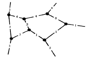
Now draw (on your own paper, because I haven't the skills to draw it nicely here) the dual diagram, which consists of (except at the edges) a bunch of triangles, and think of the labels on its edges as lengths. You'll see that each triangle is possible, in that its edges obey the triangle inequality (although many of them are degenerate and, even accounting for that, the diagram cannot be embedded in Euclidean space).

Now go back to the original diagram and redraw it so that the label becomes the number of edges between the neighbouring pair. If you want to cross from one region to another, its difficulty (as measured by the number of pipes that you have to jump over) is given by the label in the dual diagram. (The other thing that you can do with this diagram is connect all of the pipes up in a unique way. This relies on a parity condition in addition to the triangle inequality.)

Posted by: Toby Bartels on November 4, 2009 9:46 PM | Permalink | Reply to this

Re: An Adventure in Analysis

Toby! That is awesome! :)

Maybe another way to think of it is that each “wire” has a given thickness and the number of wires determines the total thickness of the edge, which corresponds to the length of the dual edge. If you allow the thick edges to overlap, they will be just thick enough to completely cover the plane.

I don’t remember seeing the relationship between the conservation law and the triangle inequality enunciated so clearly like that (although I’m sure I’ve seen it). Very neat.

I’m sure the same idea applies to higher dimensions. For example with a tetrahedron, the sum of the 4 “area vectors” should be zero. The dual edge to each triangle should carry the area of the triangle

This reminds me of a wild idea I had in grad school related to Regge calculus. But then THAT is interesting because Regge calculus is about “deficit angles” which are somehow related to Tom’s “weights” so maybe there is some connection here.

Posted by: Eric Forgy on November 4, 2009 10:03 PM | Permalink | Reply to this

Re: An Adventure in Analysis

I don’t remember seeing the relationship between the conservation law and the triangle inequality enunciated so clearly like that (although I’m sure I’ve seen it). Very neat.

I'm glad you like it. I learned all of this stuff in the the very first term of John's Quantum Gravity seminar (from back when it was really about quantum gravity), in Track 1 around Week 8. Maybe you saw it on sci.physics.research then.

Posted by: Toby Bartels on November 4, 2009 10:29 PM | Permalink | Reply to this

Re: An Adventure in Analysis

Somewhere on spr is a long post of mine where I worked some of this stuff out for some small finite group. Unfortunately, I’ve forgotten so much that I not only couldn’t remember how the Poincaré dual came into it in my post above, I also can’t even work out what would be some useful search terms to dig it out. :-(

Or Eric could look at the qg seminar, or John’s spin networks paper, since those were my starting point too.

Posted by: Tim Silverman on November 4, 2009 10:56 PM | Permalink | Reply to this

Re: An Adventure in Analysis

Somewhere on spr is a long post of mine

That’s what I mean. Posts to discussion forums and blogs tend to disappear after a while. If not in principle, but in practice. It’s a pity.

Posted by: Urs Schreiber on November 5, 2009 12:27 PM | Permalink | Reply to this

Re: An Adventure in Analysis

True true. SPR contains a true wealth of knowledge, but I don’t remember the last time I found myself there (aside from a special recent case when Toby transferred some material to the nLab from an old conversation at SPR about fancy shmancy forms :))

Then again, in 20 years, we’ll probably say the same thing about the nLab…

Posted by: Eric Forgy on November 5, 2009 3:17 PM | Permalink | Reply to this

Re: An Adventure in Analysis

Then again, in 20 years, we’ll probably say the same thing about the nLab…

Why do you say that? This I doubt. The wiki format with its entry names and cross links is precisely there to form a useful database of knowledge. That’s the reason why we are keeping information there instead of losing it on a blog.

I mean, things like Wikipedia are there to organize material such that it can be found. Right? That’s the whole point.

Posted by: Urs Schreiber on November 5, 2009 4:05 PM | Permalink | Reply to this

Re: An Adventure in Analysis

Back when we were on SPR, with the technology available to us and the state of knowledge back then, participants probably thought, “Hey! We FINALLY have something permanent. Something easily searchable with subject names and cross links.”

Then we moved to blogs. When we started the blogs, we probably thought, “Hey! We FINALLY have something that is going to be permanent. Something complete with subject names and cross links, etc.”

Now we are moving to the nLab and we think, “Hey! We FINALLY have something permanent. Complete with entry names and cross links.”

Today, SPR is STILL a valuable resource if you want it to be. The blog is STILL a valuable resource. Twenty years from now, the nLab will STILL be a valuable resource, but we will likely have moved on to something different by that time. What it is, I can’t imagine. I wish I could :)

Posted by: Eric Forgy on November 5, 2009 4:26 PM | Permalink | Reply to this

Re: An Adventure in Analysis

OK, it’s here. Not lost at all.

Raspberry

It’s the same thread where you announced your paper with Eric, in fact.

Posted by: Tim Silverman on November 5, 2009 6:28 PM | Permalink | Reply to this

Re: An Adventure in Analysis

I’m glad you like it. I learned all of this stuff in the the very first term of John’s Quantum Gravity seminar (from back when it was really about quantum gravity), in Track 1 around Week 8. Maybe you saw it on sci.physics.research then.

Yes! That’s it. I LOVED the quantum gravity seminars :)

Posted by: Eric Forgy on November 4, 2009 11:19 PM | Permalink | Reply to this

Re: An Adventure in Analysis

Ah, yes, thanks Toby. I should have remembered that. I’ve forgotten more of this than I’d realised.

Posted by: Tim Silverman on November 4, 2009 10:52 PM | Permalink | Reply to this

Re: An Adventure in Analysis

This is interesting. Well, I have always wanted to see a kind of qft-style “propagator” or “Green’s function” interpretation of the magnitude of metric spaces, so I’m definitely in the same school of ideas as Eric.

How about the following attempt to interpret magnitude in terms of quantum-mechanical mumbo-jumbo. I hope experts on this stuff here at the n-category cafe will help me out, since my quantum field theory can be dodgy at the best of times!

So we have nn points M={a i}M = \{a_i\} sitting inside m\mathbb{R}^m, and we define Z ij=exp(d(a i,a j))Z_{ij} = \exp(-d(a_i, a_j)). We want to interpret the “magnitude” of that bunch of points, namely the expression

(1)Magnitude(M)= iZ ii 1. Magnitude(M) = \sum_i Z^{-1}_{ii}.

Well, if I look at page 9 of these notes on Gaussian integrals in quantum field theory, we see that we can use “Wick’s theorem” to interpret the magnitude of MM as the expectation value of the squared distance from the origin:

(2)||x|| 2 ix i 2:=dx 1dx n[ ix i 2]e 12x TZx \langle || x ||^2 \rangle \equiv \langle \sum_i x_i^2 \rangle := \int dx_1 \ldots dx_n [\sum_i x_i^2] e^{-\frac{1}{2}x^T Z x}

That is to say, we use the points {a i}\{a_i\} to define a new inner product on n\mathbb{R}^n, via x,y=x tZy\langle x, y \rangle = x^t Z y, following which the magnitude of MM is now interpreted as the expectation value of the squared distance from the origin with respect to this new inner product.

(Maybe another way of looking at it would be to view the magnitude as (a constant times) the volume of the unit sphere with respect to this new inner product on n\mathbb{R}^n?)

Anyway, I’m not sure if this helps at all, but one thing it does do is give us a way to embed the original problem (say, an abstract finite metric space MM such that Z ij=exp(d(i,j))Z_{ij} = \exp(-d(i,j)) is positive definite) into a n\mathbb{R}^n type context, so that suddenly we can think about the abstract magnitude of MM as being about the concrete expectation value of the distance-from-the-origin-squared inside a concrete n\mathbb{R}^n.

Maybe there’s other qft-style ways of looking at this? Perhaps one could start talking about “matrix integrals”, like in these notes. Perhaps these would come in if one was interested in somehow integrating over all metrics on that finite set of points.

Posted by: Bruce Bartlett on November 4, 2009 7:30 PM | Permalink | Reply to this

Re: An Adventure in Analysis

Shouldn’t you have

Magnitude(M)= ijZ ij 1? Magnitude(M) = \sum_{i j} Z_{i j}^{-1} ?

Posted by: David Corfield on November 4, 2009 7:49 PM | Permalink | Reply to this

Re: An Adventure in Analysis

Woops! Yes, you’re right. Also didn’t put in the normalizing factor. Well, we’re left with

(1)Magnitude(M)= i,jx ix j=(2πdetZ) n2 i,jdx 1dx nx ix jexp(12x tZx) Magnitude(M) = \sum_{i,j} \langle x_i x_j \rangle = \left( \frac{2\pi}{\det Z} \right)^{\frac{n}{2}} \sum_{i,j} \int dx_1 \cdots dx_n x_i x_j exp(-\frac{1}{2}x^t Z x)

which doesn’t seem very illuminating.

Posted by: Bruce Bartlett on November 4, 2009 10:06 PM | Permalink | Reply to this

Re: An Adventure in Analysis

Covariance is defined by

cov(x i,x j)=x ixjx ix j.\cov(x_i,x_j) = \langle x_ix_j\rangle - \langle x_i\rangle\langle x_j\rangle.

It looks like x i,x j=0\langle x_i\rangle,\langle x_j\rangle = 0 so

cov(x i,x j)=x ix j.\cov(x_i,x_j) = \langle x_i x_j\rangle.

If we let

x= ix ix = \sum_i x_i

then

Magnitude(M)=cov(x,x)=x 2,Magnitude(M) = \cov(x,x) = \|x\|^2,

i.e. the magnitude of MM is the variance of xx.

Warning: I’m computing without thinking. Never a good idea. Long day :)

Posted by: Eric Forgy on November 4, 2009 11:02 PM | Permalink | Reply to this

Re: An Adventure in Analysis

i.e. the magnitude of M is the variance of x.

Ok, but I can’t think of a nice interpretation for the expression x= ix ix = \sum_i x_i.

Posted by: Bruce_Bartlettt on November 5, 2009 8:41 AM | Permalink | Reply to this

Re: An Adventure in Analysis

I was giving my brain cramps thinking about this stuff a while back and came to the idea that maybe we should be thinking about multisets. Multisets form a rig and the multiset x= ix ix = \sum_i x_i is the “unit multiset” in the free rig generated by x ix_i. That is on my doodle page. The neat thing about that is then we have

Magnitude(M)=𝟙 2.Magnitude(M) = \|\mathbb{1}\|^2.

As usual, beware I haven’t had my coffee yet.

Posted by: Eric Forgy on November 5, 2009 2:49 PM | Permalink | Reply to this

Re: An Adventure in Analysis

By the way, after prior discussions I started doodling some related ideas here. Feedback welcome!

Posted by: Eric Forgy on November 4, 2009 8:02 PM | Permalink | Reply to this

Re: An Adventure in Analysis

This is for anyone who downloaded the detailed version and was as dismayed as I was about the state of the Appendix, which shows that the functions e 2πi,xe^{2\pi i \langle -, \mathbf{x}\rangle} on n\mathbb{R}^n (x n\mathbf{x} \in \mathbb{R}^n) are linearly independent.

Mark Meckes pointed out that this is an instance of a well-known fact, ‘linear independence of characters’. Indeed, I even taught the same argument to undergraduates, two years running, in a Galois Theory course. I’ve now updated the detailed version to take advantage of this improved, shorter proof.

Posted by: Tom Leinster on November 7, 2009 1:40 AM | Permalink | Reply to this
Read the post Magnitude of Metric Spaces: A Roundup
Weblog: The n-Category Café
Excerpt: Resources on magnitude of metric spaces.
Tracked: January 10, 2011 4:01 PM

Post a New Comment