The n-Category Café

Division into Sectors

Recall that we get from $X(N)$ to $X_1(N)$ by cutting out a sector of the former, like an orange, or a pizza, and identifying the left and right edges with each other, to give the latter. The sector has its tip at the centre of the $N$-gon $\frac{1}{0}$, and it occupies a $\frac{1}{N}$th of a full $360^\circ$.

We’ve seen this with the $N\le 5$ cases, where we divide the surface of a sphere into sectors. Now we’re moving up to $X(6)$, of genus $1$. So let’s take the tiling of the plane that we use to show $X(6)$, and divide it into $6$ sectors centred at $\frac{1}{0}$.

Since images of $\frac{1}{0}$ appear in a regular lattice, so do the sectors! Notice however that each central hexagon $\frac{1}{0}$ appears three times in each triangular section. Of course, these get identified with each other when we quotient by the lattice to form a torus, but we can get a clearer idea of what exactly appears in $X_1(6)$ by dividing each triangle into three, for instance like this:

Or, putting all divisions on an equal footing:

And looking more closely at one cell:

For each denominator, observe what fraction of a complete hexagon ends up being assigned to that denominator.

• We get $1$ sixth of the hexagon with denominator $0$ (at the bottom).

• For the hexagon with denominator $1$, directly above it, we get to keep the whole hexagon—all $6$ sixths of it.

• For denominator $2$, the two parts coming from (in this picture) $\frac{3}{2}$ and $\frac{1}{2}$ add up to $3$ sixths of a whole hexagon.

• Finally, for denominator $3$, the hexagon at the top, our sector gets assigned $2$ sixths of the whole hexagon.

In short, for denominator $d$, there were a total $\frac{N}{d}$ original hexagons in $X(N)$, and for the same denominator $d$ we get $\frac{N}{d}$ sixths of a hexagon in $X_1(N)$: all types of hexagon get divided equally into six.

And this is generally true for arbitrary $N$: however many $N$-gons there were for a denominator $d$ in $X(N)$—say, $M_d$—we get the same number, $M_d$, of sectors of an $N$-gon—the same number of $N$ths of an $N$-gon—for denominator $d$ in $X_1(N)$.

So let’s cut out one of these little sectors and roll it up, as we did with the $N\lt 6$ cases last time, and see what we get!

Once again, the shape rolls into a sort of cone. Rather than generating this picture programmatically, I made one out of paper, seeing as this seemed easier:

I’ve labelled each section by its denominator, and pointed out the seams where I sellotaped together identified the left and right edges of the kite shape, with a right angle between the long and short edges of the kite. Note that although there are three conical points on this model, these are all the locations of cusps, so not really elliptic points at all.

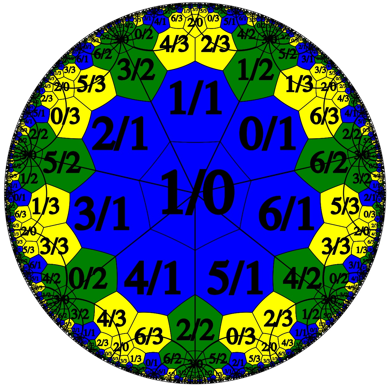
Now we’ll take a look at the case $N=7$. Here is the tiling with lines marking the sectors:

We can see that we have one sector of a heptagon for each of $\frac{1}{0}$, $\frac{2}{0}$ and $\frac{3}{0}$, and a whole heptagon for each of the denominators $1$, $2$ and $3$, though in the latter two cases they appear to be split across two heptagons until we remember to identify the left and right sides.

(I apologise that there aren’t enough lines going through $\frac{2}{0}$. All these lines originate in faces with $\frac{1}{0}$ in the centre, and the method I’ve been using to generate these pictures can’t be persuaded to generate enough such faces without more care and attention that I have free to devote to it. Fortunately that doesn’t have any ill effects on our ability to identify a unit cell.)

Looking carefully, we see that, like $X(7)$, $X_1(7)$ can be divided into three identical pieces. Here, we’ve coloured them differently:

Labelling the Edges of the $N$-gons

I’m interested in saying something about how the three pieces of this curve—the blue piece, the green piece and the yellow piece—fit together. The relationship (at least for this $N=7$ case) isn’t too complicated. We need to consider how the edges of the various parts are related—which edges are glued to which other edges.

Look at the sector vertically above the centre of the picture. There’s one $7$th of the $\frac{1}{0}$ heptagon, which will roll into a cone (whose conical tip is not a genuinely special point, although it appears so in this model). Above that is the $\frac{1}{1}$ heptagon.

Let’s consider the edges of the $\frac{1}{1}$ heptagon, carefully taking note of which coloured pieces adjoin to which other coloured pieces. In order to understand this better, I’ve labelled its edges, starting with $0$ along the edge in contact with the $\frac{1}{0}$ cone and increasing as we move away. And I’ve labelled the edges of the other two heptagons correspondingly:

• The bottom edge of $\frac{1}{1}$, which is joined to $\frac{1}{0}$, (let’s call that “edge-$0$”) forms a loop, with its two ends identified, once the left and right sides of the sector have been identified.

• The next pair of edges— the edges adjacent to $\frac{2}{1}$ and $\frac{0}{1}$—get identified with each other, rolling the heptagon up into a tube. This happens because these edges are adjacent to other blue heptagons—i.e. heptagons with denominator $1$—and all heptagons with denominator $1$ get identified with each other. Let’s call those edges the left and right “edge-$1$”.

• The edges adjacent to $\frac{3}{2}$ and $\frac{1}{2}$—let’s call them the left and right “edge-$2$” of this heptagon—obviously end up joined to two edges of the green piece (i.e. the piece with a denominator of $2$ in its main body and $\frac{3}{0}$ at its conical tip).

• Finally, the next edges along on the blue heptagon, viz. the left and right “edge-$3$”, join to the yellow piece, with a denominator of $3$ in its main body and $\frac{2}{0}$ at its tip.

But what is going on on the other sides of those edges? For instance, how about on the other side of edge-$2$, in the green piece?

We can number the edges of the green piece in the same way, beginning with $0$ adjacent to the denominator-$0$ tip and working outwards. By the time we get to the blue piece, and the edge that is numbered $2$ on the blue side, we have reached $3$ on the green side.

And likewise, moving to edge-$3$ of the blue piece, and crossing to the other side, we find that we are at edge-$2$ of the yellow denominator-$3$ heptagon.

And finally, the edge-$2$ of the green heptagon is joined to the edge-$3$ of the yellow heptagon.

To generalise over the blue, green and yellow pieces:

• each piece consists of one sector with denominator $\frac{u}{0}$ rolled into a cone, attached to a whole heptagon with denominator $\frac{1}{u}$, rolled into a tube. (E.g. the sector $\frac{2}{0}$ is adjacent to the heptagon with denominator $\frac{1}{2}=3$.)

• The first edge of the whole heptagon (edge-$0$) is curled round to join its two ends together, and attaches to the base of the cone.

• The two edges of the heptagon adacent to that (the left and right versions of edge-$1$) are joined to each other to form a seam.

• The next edges—the left and right edge-$2$—are joined onto the edge-$3$s of one of the other two pieces.

• The next edges, the edge-$3$s, join each other at their ends to form a pointed tip; and they are joined to the edge-$2$s of the second of the other two pieces in the complete curve.

To summarise the summary, the edge-$2$s of one heptagon are joined to the edge-$3$s of another heptagon, in a cyclic manner ($1\rightarrow 2\rightarrow 3\rightarrow 1$).

I made a model of $X_1(7)$ out of paper too. Since plane heptagons have angles quite close to $120^\circ$, I could get away with using flat paper rather than “hyperbolic paper” which I don’t seem to be able to lay my hands on just now. I’ve left off the conical tips and just included the heptagons with non-$0$ denominator:

The heptagons are labelled by denominator. I’ve noted the edge in each piece which is wrapped around to form a “loop” (and in the full curve would join to a denominator-$0$ cone). I’ve also noted the “seams” where the edge-$1$s are identified with each other. If you look closely, you can also mostly see where I labelled the edges “$0$”, “$1$” and “$2$” (in order to help me put the model together correctly). But be warned! these correspond to the “edge-$1$”, “edge-$2$” and “edge-$3$” (respectively) defined in the previous paragraphs—they are due to an earlier, and inferior, numbering scheme! However, they should at least make it clear that $2$-edges join to $3$-edges cyclically. It’s obvious that the curve has a $3$-fold rotational symmetry, corresponding to the action of the projective group of units, which is isomorphic to $\mathbb{Z}_3$.

The curve is mirror-symmetric in a plane parallel to the plane of the page, corresponding to the mirror symmetry about the bisector of the sectors(!), e.g. about the vertical axis in the earlier picture. Note that it is not mirror-symmetric across any plane including the axis of rotational symmetry—it has a handedness. (I think the choice of handedness in representing the curve in (e.g.) a paper model ultimately goes back to the choice of orientation of our representation of the complex plane—i.e. our decision that $i$ lies $90^\circ$ anticlockwise of $1$, and $-i$ lies $90^\circ$ clockwise, rather than the other way round.)

More general $N$

Next time I’ll attempt to draw some surfaces $X_1(N)$ for $N\gt 7$. But for the moment, I won’t be able to reveal anything very beautiful about the geometry of these cases. Instead I’ll try to sketch an impression by concentrating on arithmetic. Like $X(N)$, these surfaces divide into a set of identical blocks, the same in number as the order of the projective group of units, which indeed acts to permute them. The blocks each consist of a cone made from one sector of a denominator-$0$ $N$-gon, attached to a full $N$-gon which is rolled up into a tube with one edge (“edge-$0$”) joined to the denominator-$0$ cone, the “edge-$1$s” on either side of that glued to each other, and then either a simple linear succession of pairs of edges (edge-$2$s, edge-$3$s, edge-$4$s, etc) glued to other blocks (in the case of $N$ prime) or something similar but more complicated (for $N$ composite). In particular, for $N$ prime, the projective group of units is always cyclic, so the blocks are arranged like some kind of complicated toy windmill with $\frac{N-1}{2}$ blades, of which the two-blade windmill called $X_1(5)$ and the three-blade windmill called $X_1(7)$ are the simplest examples.

Orbits under Translation

I’ll try to describe the main features of the “something more complicated” for composite $N$. If you think back a couple of posts, you’ll recall I was discussing the orbits of fractions under the action of the group of rescalings. We classified the orbits according to the gcd of the denominator with $N$—that is, into one class for each factor of $N$. For example, for $N=15$, here are the fractions $\frac{p}{q}$ with $(q,N)=3$, organised into orbits: each orbit is a column, and the matrix giving the rescaling action labels the row to its right.

$\array{\arrayopts{\collines{solid}\frame{solid}}\left(\array{1&0\\0&1}\right)& \frac{1}{3}&\frac{2}{3}&\frac{4}{3}&\frac{5}{3}&\frac{8}{3}\\ \left(\array{8&0\\0&2}\right)& \frac{8}{6}&\frac{1}{6}&\frac{2}{6}&\frac{10}{6}&\frac{4}{6}\\ \left(\array{4&0\\0&4}\right)& \frac{11}{3}&\frac{7}{3}&\frac{14}{3}&\frac{10}{3}&\frac{13}{3}\\ \left(\array{13&0\\0&7}\right)& \frac{13}{6}&\frac{11}{6}&\frac{7}{6}&\frac{5}{6}&\frac{14}{6}}$

The number of rows is of course the order of the projective group of units.

We also worked out a formula for the number of columns—the number of orbits—for a given factor $d\vert N$, which I’ll repeat for reference, as follows:

But there is another completely different way to arrange the same fractions into a rectangle (often but not always with the same number of rows and the same number of columns), based not on permuting the fractions in a column by the action of rescalings (multiplication by an invertible constant) but on permuting the fractions in a row by the action of translations (addition of any constant). For example, the same fractions as above now look like the following:

$\array{\arrayopts{\rowlines{solid}\frame{solid}}\frac{1}{3}&\frac{4}{3}&\frac{7}{3}&\frac{10}{3}&\frac{13}{3}\\ \frac{1}{6}&\frac{7}{6}&\frac{13}{6}&\frac{4}{6}&\frac{10}{6}\\ \frac{2}{3}&\frac{5}{3}&\frac{8}{3}&\frac{11}{3}&\frac{14}{3}\\ \frac{2}{6}&\frac{8}{6}&\frac{14}{6}&\frac{5}{6}&\frac{11}{6}}$

Now, adding $1$ shifts everything one space to the right.

(The relationship between the two arrangements varies depending on $N$. I haven’t looked into it deeply.)

The effect of going from $X(N)$ to $X_1(N)$ is precisely to collapse each of these rows horizontally into one element. Geometrically, some number of $N$-gons gets identified; but, more than that, that $N$-gon will usually be further quotiented by some fraction of a turn. For instance, in the above case, we are quotienting by a group of order $15$ (viz. $\mathbb{Z}_{15}$) but there are only $5$ fractions per row, so the $5$ pentadecagons reduce to a third of $1$ pentedecagon—a conical shape with $5$ triangular sectors. In fact, in general, we get the same number of triangular sectors in one cone (or complete $N$-gon) as there were originally $N$-gons in the row. Each row contributes one cone (and hence one cusp). However, because the actual arrangement of fractions between rows is generally different in the two arrangements I’ve been talking about (actions by rescaling within columns and actions by translating within rows), sectors of the same cone may end up being divided between different pieces of the curve.

Let’s quickly calculate the number of cusps for a given factor $d\vert N$.

In general, the number of columns in this system is $\frac{N}{d}$, so we divide each term in $p_i$ by $p_i^{n_i-m_i}$. We can calculate the total number of fractions in the rectangle based on the first arrangement, bearing in mind that the projective units of $\mathbb{Z}_N$ gives rise to a contribution of $p_i^{n_i}-p_i^{n_i-1}$, (with an overall factor of $\frac{1}{2}$ outside the product over $i$). Hence we have:

For $m=0$

$(p_i^{n_i}-p_i^{n_i-1})\cdot p_i^{n_i-m_i}\cdot p_i^{-(n_i-m_i)}=p_i^{n_i}-p_i^{n_i-1}$.

For $0\lt m_i\lt n_i$

$(p_i^{n_i}-p_i^{n_i-1})\cdot(p_i^{n_i-m_i}-p_i^{n_i-m_i-1})\cdot p_i^{-(n_i-m_i)}=(p_i^{n_i-1}-p_i^{n_i-2})(p-1)$.

For $m_i=n_i$

$(p_i^{n_i}-p_i^{n_i-1})\cdot 1\cdot 1=p_i^{n_i}-p_i^{n_i-1}$.

Overall, we have

$p_i^{n_i-2}(p-1)\cdot\thinspace\left\{\array{p\(p-1)}\right.\thickspace for \left\{\array{m_i=0\thinspace or m_i=n_i\0\lt m_i\lt n_i}\right.$</p> <p>Another complication, which I will expand in an example a little later, is that although$X_1(N)$is mirror symmetrical in a plane, it does not follow that edges on the left side only join to other edges on the left side: there can be joins across the centre line, and, as a consequence, the curves$X_1(N)$can have non-$0$genus (as, of course, can the curves$X(N)$).

Next time, there will be more pretty pictures and a lot less arithmetic.