Skip to the Main Content

Note:These pages make extensive use of the latest XHTML and CSS Standards. They ought to look great in any standards-compliant modern browser. Unfortunately, they will probably look horrible in older browsers, like Netscape 4.x and IE 4.x. Moreover, many posts use MathML, which is, currently only supported in Mozilla. My best suggestion (and you will thank me when surfing an ever-increasing number of sites on the web which have been crafted to use the new standards) is to upgrade to the latest version of your browser. If that's not possible, consider moving to the Standards-compliant and open-source Mozilla browser.

June 29, 2015

Feynman’s Fabulous Formula

Posted by Simon Willerton

Guest post by Bruce Bartlett.

There is a beautiful formula at the heart of the Ising model; a formula emblematic of all of quantum field theory. Feynman, the king of diagrammatic expansions, recognized its importance, and distilled it down to the following combinatorial-geometric statement. He didn’t prove it though — but Sherman did.
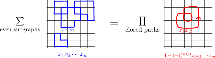
Feynman’s formula. Let GG be a planar finite graph, with each edge ee regarded as a formal variable denoted x ex_e. Then the following two polynomials are equal:

H evenGx(H)= [γ]P(G)(1(1) w[γ]x[γ])\displaystyle \sum_{H \subseteq_{even} G} x(H) = \prod_{[\vec{\gamma}] \in P(G)} \left(1 - (-1)^{w[\vec{\gamma}]} x[\vec{\gamma}]\right)

pic

I will explain this formula and its history below. Then I’ll explain a beautiful generalization of it to arbitrary finite graphs, expressed in a form given by Cimasoni.

What the formula says

The left hand side of Feynman’s formula is a sum over all even subgraphs HH of GG, including the empty subgraph. An even subgraph HH is one which has an even number of half-edges emanating from each vertex. For each even subgraph HH, we multiply the variables x ex_e of all the edges eHe \in H together to form x(H)x(H). So, the left hand side is a polynomial with integer coefficients in the variables x e ix_{e_i}.

The right hand side is a product over all γP(G)\vec{\gamma} \in P(G), where P(G)P(G) is the set of all prime, reduced, unoriented, closed paths in GG. That’s a bit subtle, so let me define it carefully. Firstly, our graph is not oriented. But, by an oriented edge e\mathbf{e}, I mean an unoriented edge ee equipped with an orientation. An oriented closed path γ\vec{\gamma} is a word of composable oriented edges e 1e n\mathbf{e_1} \cdots \mathbf{e_n}; we consider γ\vec{\gamma} up to cyclic ordering of the edges. The oriented closed path γ\vec{\gamma} is called called reduced if it never backtracks, that is, if no oriented edge e\mathbf{e} is immediately followed by the oriented edge e 1\mathbf{e^{-1}}. The oriented closed path γ\vec{\gamma} is called prime if, when viewed as a cyclic word, it cannot be expressed as the product δ r\vec{\delta}^r of a given oriented closed path δ\vec{\delta} for any r2r \geq 2. Note that the oriented closed path γ\vec{\gamma} is reduced (resp. prime) if and only if γ 1\vec{\gamma}^{-1} is. It therefore makes sense to talk about prime reduced unoriented closed paths [γ][\vec{\gamma}], by which we mean simply an equivalence class [γ]=[γ 1][\vec{\gamma}] = [\vec{\gamma}^{-1}].

Suppose GG is embedded in the plane, so that each edge forms a smooth curve. Then given an oriented closed path γ\vec{\gamma}, we can compute the winding number w(γ)w(\vec{\gamma}) of the tangent vector along the curve. We need to fix a convention about what happens at vertices, where we pass from the tangent vector vv at the target of e i\mathbf{e_i} to the tangent vector vv' at the source of e i+1\mathbf{e_{i+1}}. We choose to rotate vv into vv' by the angle less than π\pi in absolute value.

Note that w(γ)=w(γ)w(-\vec{\gamma}) = -w(\vec{\gamma}), so that its parity (1) w[γ](-1)^{w[\vec{\gamma}]} makes sense for unoriented paths. Finally, by x[γ]x[\vec{\gamma}] we simply mean the product of all the variables x e ix_{e_i} for e ie_i along γ\vec{\gamma}.

The product on the right hand side is infinite, since P(G)P(G) is infinite in general (we will shortly do some examples). But, we regard the product as a formal power series in the terms x e 1x e 2x e nx_{e_1} x_{e_2} \cdots x_{e_n}, each of which only receives finitely many contributions (there are only finitely many paths of a given length), so the right hand side is a well-defined formal power series.

Examples

Let’s do some examples, taken from Sherman. Suppose GG is a graph with one vertex vv and one edge ee:

pic

Write x=x(e)x = x(e). There are two even subgraphs — the empty one, and GG itself. So the sum over even subgraphs gives 1+x1+x. There is only a single closed path in P(G)P(G), namely [e][\mathbf{e}], with odd winding number, so the sum over paths also gives 1+x1+x. Hooray!

Now let’s consider a graph with two loops:

pic

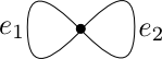
There are 4 even subgraphs, and the left hand side of the formula is 1+x 1+x 2+x 1x 21 + x_1 + x_2 + x_1x_2. Now let’s count closed paths γP(G)\gamma \in P(G). There are infinitely many; here is a table. Let e 1\mathbf{e_1} and e 2\mathbf{e_2} be the counterclockwise oriented versions of e 1e_1 and e 2e_2. [γ] 1(1) w[γ]x[γ] [e 1] 1+x 1 [e 2] 1+x 2 [e 1e 2] 1+x 1x 2 [e 1e 2 1] 1x 1x 2 [e 1 2e 2] 1x 1 2x 2 [e 1 2e 2 1] 1+x 1 2x 2 [e 1e 2 2] 1x 1x 2 2 [e 1 1e 2 2] 1+x 1x 2 2 \begin{array}{cc} [\vec{\gamma}] & 1 - (-1)^{w[\vec{\gamma}]} x[\vec{\gamma}] \\ ------ & ------ \\ [\mathbf{e_1}] & 1 + x_1 \\ [\mathbf{e_2}] & 1 + x_2 \\ [\mathbf{e_1 e_2}] & 1 + x_1 x_2 \\ [\mathbf{e_1 e_2^{-1}}] & 1 - x_1 x_2 \\ [\mathbf{e_1^2 e_2}] & 1 - x_1^2 x_2 \\ [\mathbf{e_1^2 e_2^{-1}}] & 1 + x_1^2 x_2 \\ [\mathbf{e_1 e_2^2}] & 1 - x_1 x_2^2 \\ [\mathbf{e_1^{-1} e_2^2}] & 1 + x_1 x_2^2 \\ \cdots & \cdots \end{array} If we multiply out the terms the right hand side gives (1+x 1+x 2+x 1x 2)(1x 1 2x 2 2)(1x 1 4x 2 2)(1x 1 2x 2 4) (1 + x_1 + x_2 + x_1 x_2) (1-x_1^2 x_2^2) (1-x_1^4 x_2^2)(1-x_1^2x_2^4) \cdots In order for this to equal 1+x 1+x 2+x 1x 2 1 + x_1 + x_2 + x_1x_2 we will need some miraculous cancellation in the higher powers to occur! And indeed this is what happens. The minus signs from the winding numbers conspire to cancel the remaining terms. Even in this simple example, the mechanism is not obvious — but it does happen.

Pondering the meaning of the formula

Let’s ponder the formula. Why do I say it is so beautiful?

Well, the left hand side is combinatorial — it has only to do with the abstract graph GG, having the property that it is embeddable in the plane (this property can be abstractly encoded via Kuratowski’s theorem). The right hand side is geometric — we fix some embedding of GG in the plane, and then compute winding numbers of tangent vectors! So, the formula expresses a combinatorial (or topological) property of the graph in terms of geometry.

Ok… but why is this formula emblematic of all of quantum field theory? Well, summing over all loops is what the path integral in quantum mechanics is all about. (See Witten’s IAS lectures on the Dirac index on manifolds, for example.) Note that the quantum mechanics path integral has recently been made rigorous in the work of Baer and Pfaffle, as well as Fine and Sawin.

Also, I think the formula has overtones of the linked-cluster theorem in perturbative quantum field theory, which relates the generating function for all Feynman diagrams (similar to the even subgraphs) to the generating function for connected Feynman diagrams (similar to the closed paths). You can see why Feynman was interested!

History of the formula

One beautiful way of computing the partition function in the Ising model, due to Kac and Ward, is to express it as a square root of a certain determinant. (I hope to explain this next time.) To do this though, they needed a “topological theorem” about planar graphs. Their theorem was actually false in general, as shown by Sherman. It was Feynman who reformulated it in the above form. From Mark Kac’s autobiography (clip):

The two-dimensional case for so-called nearest neighbour interactions was solved by Lars Onsager in 1944. Onsager’s solution, a veritable tour de force of mathematical ingenuity and inventiveness, uncovered a number of suprising features and started a series of investigations which continue to this day. The solution was difficult to understand and George Uhlenbeck urged me to try to simplify it. “Make it human” was the way he put it …. At the Institute [for Advanced Studies at Princeton] I met John C. Ward … we succeeded in rederiving Onsager’s result. Our success was in large measure due to knowing the answer; we were, in fact, guided by this knowledge. But our solution turned out to be incomplete… it took several years and the effort of several people before the gap in the derivation was filled. Even Feynman got into the act. He attended two lectures I gave in 1952 at Caltech and came up with the clearest and sharpest formulation of what was needed to fill the gap. The only time I have ever seen Feynman take notes was during the two lectures. Usually, he is miles ahead of the speaker but following combinatorial arguments is difficult for all mortals.

Feynman’s formula for general graphs

Every finite graph can be embedded in some closed oriented surface of high enough genus. So there should be a generalization of the formula to all finite graphs, not just planar ones. But on the right hand side of the formula, how do we compute the winding number of a closed path on a general surface? The answer, in the formulation of Cimasoni, is beautiful: we should sum over spin structures on the surface, each weighted by their Arf invariant!

Generalized Feynman formula. Let GG be a finite graph of genus gg. Then the following two polynomials are equal: H evenGx(H)=12 g λSpin(Σ)(1) Arf(λ) [γ]P(G)(1(1) w λ[γ]x[γ]) \sum_{H \subseteq_{even} G} x(H) = \frac{1}{2^g} \sum_{\lambda \in Spin(\Sigma)} (-1)^{Arf(\lambda)} \prod_{[\vec{\gamma}] \in P(G)} (1 - (-1)^{w_\lambda[\vec{\gamma}]} x[\vec{\gamma}])

The point is that a spin structure on Σ\Sigma can be represented as a nonzero vector field λ\lambda on Σ\Sigma minus a finite set of points, with even index around these points. (Of course, a nonzero vector field on the whole of Σ\Sigma won’t exist, except on the torus. That is why we need these points.) So, we can measure the winding number w λ(γ)w_\lambda(\vec{\gamma}) of a closed path γ\vec{\gamma} with respect to this background vector field λ\lambda.

The first version of this generalized Feynman formula was obtained by Loebl, in the case where all vertices have degree 2 or 4, and using the notion of Sherman rotation numbers instead of spin structures (see also Loebl and Somberg). In independent work, Cimasoni formulated it differently using the language of spin structures and Arf invariants, and proved it in the slightly more general case of general graphs, though his proof is not a direct one. Also, in unpublished work, Masbaum and Loebl found a direct combinatorial argument (in the style of Sherman’s proof of the planar case) to prove this general, spin-structures version.

Last thoughts

I find the generalized Feynman’s formula to be very beautiful. The left hand side is completely combinatorial / topological, manifestly only depending on GG. The right hand picks some embedding of the graph in a surface, and is very geometric, referring to high-brow things such as spin structures and Arf invariants! Who knew that there was such an elegant geometric theorem lurking behing arbitrary finite graphs?

Moreover, it is all part of a beautiful collection of ideas relating the Ising model to the free fermion conformal field theory. (Indeed, the appearance of spin structures and winding numbers is telling us we are dealing with fermions.) Of course, physicists knew this for ages, but it hasn’t been clear to mathematicians exactly what they meant :-)

But in recent times, mathematicians are making this all precise, and beautiful geometry is emerging, like the above formula. There’s even a Fields medal in the mix. It’s all about discrete complex analysis, spinors on Riemann surfaces, the discrete Dirac equation, isomonodromic deformation of flat connections, heat kernels, conformal invariance, Pfaffians, and other amazing things (here is a recent expository talk of mine). I hope to explain some of this story next time.

Posted at June 29, 2015 7:47 AM UTC

TrackBack URL for this Entry:   https://golem.ph.utexas.edu/cgi-bin/MT-3.0/dxy-tb.fcgi/2834

26 Comments & 0 Trackbacks

Re: Feynman’s Fabulous Formula

That’s clearly a fabulous formula. But why does the formula hold? Sometimes this kind of combinatorial formula can be seen as counting the same thing in two different ways. Do you know of anything similar going on here?

Posted by: Simon Willerton on June 29, 2015 3:07 PM | Permalink | Reply to this

Re: Feynman’s Fabulous Formula

In the direct approach of Loebl and Loebl-Masbaum, one can hopefully indeed see it as counting something in two different ways.

I am more familiar with Cimasoni’s approach, which is a bit indirect. But it can indeed be interpreted as computing a certain determinant in two ways.

Consider the RHS of Feynman’s formula. Instead of taking the product over all unoriented paths, we could take the square root of the product over all oriented paths, which is more natural:

RHS 2= γ(1(1) w(γ)x(γ)) RHS^2 = \prod_{\vec{\gamma}} (1- (-1)^{w(\vec{\gamma})} x(\vec{\gamma}))

Now, the key geometric fact is that winding numbers can be computed locally by adding up angle contributions along a path. That is,

(1) w(γ)= 1 nexp(iθ(e i,e i+1)/2) (-1)^{w(\vec{\gamma})} = \prod_1^n exp(i \theta(\mathbf{e}_i, \mathbf{e}_{i+1})/2)

where θ(e i,e i+1)\theta(\mathbf{e}_i, \mathbf{e}_{i+1}) is the difference in the angle going from the oriented edge e i\mathbf{e}_i to e i+1\mathbf{e}_{i+1}.

Now consider the 2|E|×2|E|2|E| \times 2|E| Kac-Ward matrix KK indexed by oriented edges of GG,

K e,e={exp(iθ(e,e)/2) ift(e)=s(e)butee 0 otherwise K_{\mathbf{e}, \mathbf{e}'} = \begin{cases} exp(i \theta(\mathbf{e}, \mathbf{e}')/2) & if t(\mathbf{e}) = s(\mathbf{e}') \,\,\,but \,\,\, \mathbf{e}' \neq -\mathbf{e} \\ 0 & otherwise \end{cases}

Now, in general, whenever you have a finite graph GG, and a weight w(e,e)w(\mathbf{e}, \mathbf{e}') associated to pairs of composable oriented edges, you can form the analagous matrix KK. There is a theorem called the Foata-Zeilberger-Bass theorem (see Section 2.1 of Loebl) which says that

det(1K)= γP(G)(1 i=1 nw(e i,e)) det(1 - K) = \prod_{\vec{\gamma} \in \vec{P}(G)} (1 - \prod_{i=1}^n w(\mathbf{e}_i, \mathbf{e}'))

Applying this theorem to our case, we see that that the square of the RHS of Feynman’s formula is a certain determinant,

RHS 2=det(1K) RHS^2 = det(1 - K)

On the other hand, this determinant can be calculated in a different way, as a sum over even subgraphs. This is done in Section 3 of Cimasoni’s paper. So:

det(1K)=LHS 2 det(1 - K) = LHS^2

and we are done. I don’t understand that calculation, but that is the basic idea I think: computing a determinant in two different ways.

Posted by: Bruce Bartlett on June 29, 2015 6:40 PM | Permalink | Reply to this

Re: Feynman’s Fabulous Formula

To prevent confusion. The Kac-Ward matrix is really the thing I was calling 1K1-K above. The thing I was calling KK above is usually called TT and is just called the “transition matrix”.

Posted by: Bruce Bartlett on October 18, 2015 10:45 PM | Permalink | Reply to this

Re: Feynman’s Fabulous Formula

This reminds me of Kasteleyn’s method. In Kasteleyn’s setting, we have a finite planar graph G with 2n vertices and the “left hand side” is MGx(M)\sum_{M \subset G} x(M) where the sum is now over dimer configurations, meaning subgraphs MM in which every vertex has degree 11. Kasteleyn’s result is that this is then equal to a (2n)×(2n)(2n) \times (2n) Pfaffian – if G is bipartite, this can be further simplified to an n×nn \times n determinant.

There are many nice examples where people diagonalize the Kasteleyn matrix, and hence express the sum over dimers as a product. So we have a sum over subgraphs of certain degrees written as a Pfaffian/determinant/product (which one depending on the details of the problem).

Moreover, there is a generalization to genus gg surfaces in this case as well, where one sums up 2 2g2^{2g} Pfaffians, one for each element in a principal homogenous space for H 1(X,/2)H^1(X, \mathbb{Z}/2).

Is there a connection here?

Posted by: David Speyer on June 29, 2015 3:26 PM | Permalink | Reply to this

Re: Feynman’s Fabulous Formula

I see that the abstract of Cimasoni’s paper promises to address this.

Posted by: David Speyer on June 29, 2015 3:29 PM | Permalink | Reply to this

Re: Feynman’s Fabulous Formula

Yes. Cimasoni essentially gives two proofs of Feynman’s formula (which is a spinoff, pun intended, of his computation of the partition function).

Both proofs start by using Bass’s theorem to express the right hand side as the square root of a determinant of a certain Kac-Ward matrix M=1KM = 1 - K as I explained above.

Then, in the first proof, he has a direct combinatorial argument for why the left hand side should also equal the square root of detM\det M.

In his second proof, he writes the left hand side, as the partition function of an associated dimer model. Then he expresses this partition function of the dimer model as the Pfaffian of a Kasteleyn matrix QQ. Then he explicitly transforms QQ into MM by a sequence of moves which does not change the determinant. And so we are done.

Posted by: Bruce Bartlett on June 29, 2015 6:53 PM | Permalink | Reply to this

Re: Feynman’s Fabulous Formula

Wow, this is really nice!

Posted by: Jamie Vicary on June 29, 2015 11:35 PM | Permalink | Reply to this

Re: Feynman’s Fabulous Formula

Thank you very much for this beautiful exposition of my work!

I take this opportunity to say that with Dima Chelkak & Adrien Kassel, we recently found an extremely simple proof of this Kac-Ward formula. This proof extends to graphs on surfaces, and it also makes more clear the connection to the Kasteleyn method for dimers mentioned above. The paper should be on the ArXiv in a couple of weeks.

Posted by: David Cimasoni on June 30, 2015 8:13 AM | Permalink | Reply to this

Re: Feynman’s Fabulous Formula

Sounds very interesting.

Posted by: Bruce Bartlett on June 30, 2015 7:01 PM | Permalink | Reply to this

Re: Feynman’s Fabulous Formula

For future reference. The new proof of Feynman’s formula that David Cimasoni referred to in the comment above indeed appeared shortly thereafter.

To do this they first prove a refined version of Feynman’s formula in Theorem 4.2, which computes the contribution of each spin structure separately. In my notation above, it says that for each λSpin(Σ)\lambda \in Spin(\Sigma),

H evenG(1) q λ[H]x(H)= [γ]P(G)(1(1) w λ[γ]x[γ]) \sum_{H \subseteq_{even} G} (-1)^{q_\lambda [H]} x(H) = \prod_{[\vec{\gamma}] \in P(G)} (1-(-1)^{w_\lambda [\vec{\gamma}]} x[\gamma])

In this formula, the new ingredient is the appearance of signs on the left hand side. Given an even subgraph HGH \subset G, consider its underlying cohomology class [H]H 1(G,/2)[H] \in H_1(G, \mathbb{Z}/2). From the work of Johnson, a spin structure λ\lambda can be regarded as a quadratic form

q λ:H 1(G,/2)/2. q_\lambda : H_1(G, \mathbb{Z}/2) \rightarrow \mathbb{Z}/2.

If we regard the spin structure λ\lambda as a vector field on Σ\Sigma with even-index zeros, then q λ([c])q_\lambda ([c]) basically counts the winding number mod 2 of λ\lambda around a curve cc representing the homology class [c][c].

To derive the generalized Feynman’s formula from thieir refined formula, all we need to do is average over all spin structures λSpin(Σ)\lambda \in Spin(\Sigma), and use a basic property of quadratic forms, equation (4.6) in their paper.

They give a short self-contained proof of the refined Feynman formula Theorem 4.2.

Posted by: Bruce Bartlett on October 18, 2015 11:16 PM | Permalink | Reply to this

Re: Feynman’s Fabulous Formula

Any relation between the RHS and the Ruelle zeta function

R ρ(s)=γdet(Idhol ρ(γ)e sl(γ))? R_\rho(s) = \underset{\gamma}{\prod} \det \left( Id - hol_\rho(\gamma) e^{-s l(\gamma)} \right)?

Posted by: David Corfield on June 30, 2015 2:54 PM | Permalink | Reply to this

Re: Feynman’s Fabulous Formula

Indeed, it looks very similar. Perhaps David Cimasoni could help us here.

Posted by: Bruce Bartlett on June 30, 2015 7:00 PM | Permalink | Reply to this

Re: Feynman’s Fabulous Formula

I had never heard of the Ruelle zeta function. It is an interesting analogy, but since this zeta function is defined for hyperbolic manifolds of odd dimensions, and we are dealing with graphs embedded in surfaces, this is probably not the right object to consider.

In Section 4.4 of the article

http://arxiv.org/pdf/1209.0951v1.pdf

I argue that the determinant of a Kac-Ward matrix for a weighted graph on a surface (with “critical weights”) should be understood as a discrete version of the ¯\overline{\partial}-torsion of the underlying Riemann surface. More precisely, Kac-Ward matrices can be twisted by U(1)U(1)-valued flat connections, and one hopes that the ratio of the determinants of two such twisted matrices converges to the ratio of the corresponding ¯\overline{\partial}-torsion. In particular, this limit should not depend on the graph we started with (universality).

This is trivially true in genus zero, and can be proven for tori as well. For higher genus, it is wide open. However, the torsion of a hyperbolic surface can be written as a Selberg zeta function, which looks very much like the Ruelle zeta function, but is defined for surfaces. I believe that this is the correct smooth analog to consider, but I do not know of any proven result in that direction.

Posted by: David Cimasoni on July 3, 2015 8:49 AM | Permalink | Reply to this

Re: Feynman’s Fabulous Formula

Ruelle zeta functions are defined more broadly than that. E.g., p.28 of Terras’s book. She does so for a function ff on a compact manifold MM equipped with a matrix-valued function on MM.

For a very simple choice of these, the Ruelle zeta function becomes the Ihara zeta function of a finite connected graph:

ζ(u)= [P](1u ν(P)) 1, \zeta(u) = \prod_{[P]} (1 - u^{\nu (P)})^{-1},

where the product is taken over primes, PP, and ν(P)\nu(P) is the length.

I should think it plausible that your RHS can be constructed for some other choices.

Posted by: David Corfield on July 3, 2015 1:29 PM | Permalink | Reply to this

Re: Feynman’s Fabulous Formula

From some notes on graph zeta functions:

For a choice of edge matrix, WW, and for a graph XX, there is defined the edge Ihara zeta function

ζ E(W,X)= [P](1N E(P)) 1, \zeta_E(W, X) = \prod_{[P]}(1 - N_E(P))^{-1},

over prime paths PP, where for a path C=a 1a 2a sC = a_1 a_2\cdots a_s,

N E(C)=w a 1a 2w a 2a 3w a sa 1 N_E(C) = w_{a_1 a_2} w_{a_2 a_3} \cdots w_{a_s a_1}

w abw_{a b} being a variable if edge aa feeds into edge bb.

Later they define a similar path zeta function.

Posted by: David Corfield on July 5, 2015 10:42 AM | Permalink | Reply to this

Re: Feynman’s Fabulous Formula

There’s clearly a relation with the Ihara (or Ihara-Selberg) zeta function and perhaps even more with the graph edge zeta function of Terras and Stark. This is mentioned in the Loeb paper but I haven’t got to that bit yet.

Posted by: Tim Silverman on July 1, 2015 8:38 AM | Permalink | Reply to this

Re: Feynman’s Fabulous Formula

From that Wikipedia page

The Ihara zeta function plays an important role in the study of free groups, spectral graph theory, and dynamical systems, especially symbolic dynamics, where the Ihara zeta function is an example of a Ruelle zeta function.

The source of which claim is a book

  • Terras, Audrey (2010). Zeta Functions of Graphs: A Stroll through the Garden. Cambridge Studies in Advanced Mathematics 128. Cambridge University Press.
Posted by: David Corfield on July 1, 2015 8:59 AM | Permalink | Reply to this

Re: Feynman’s Fabulous Formula

You’ll find many related refs in the comments to the MO-Q “Cycling through the Zeta Garden: Zeta functions for graphs, cycle index polynomials, and determinants” (https://mathoverflow.net/questions/111770/cycling-through-the-zeta-garden-zeta-functions-for-graphs-cycle-index-polynomi)

Posted by: Tom Copeland on January 17, 2021 9:32 PM | Permalink | Reply to this

Re: Feynman’s Fabulous Formula

Hallo, recently I proved a generalization of the Feynman formula (see 1503.02525). It shows how to write weight enumerator of any binary linear code, in particular Ising partition function of any graph, as a single product, over ‘closed walks’ in 4-uniform hypergraphs.

Posted by: Martin Loebl on July 2, 2015 8:26 PM | Permalink | Reply to this

Re: Feynman’s Fabulous Formula

Hi Martin - yes I had a look at this paper, very interesting. In the paper you view the fact that, on a general surface, the generalized Feynman formula is a sum of signed products (as opposed to a single product), as a disadvantage. Because it complicates taking the logarithm, to get the free energy. This was your motivation - to remove the sum.

But I see that sum (over spin structures) not as a disadvantage but actually as something natural, something geometric, which ties in closely with the physics approach in conformal field theory, where that sum over spin structures comes out naturally too. I wonder if you could comment on this.

Posted by: Bruce Bartlett on July 6, 2015 1:30 PM | Permalink | Reply to this

Re: Feynman’s Fabulous Formula

You will probably find this paper interesting too.

http://www.sciencedirect.com/science/article/pii/S0166218X09000821

Posted by: Jonas on August 16, 2015 11:53 AM | Permalink | Reply to this

Re: Feynman’s Fabulous Formula

Working a readable link:

The bivariate Ising polynomial of a graph by Andrén and Markström.

Abstract:

In this paper we discuss the two variable Ising polynomials in a graph theoretical setting. This polynomial has its origin in physics as the partition function of the Ising model with an external field. We prove some basic properties of the Ising polynomial and demonstrate that it encodes a large amount of combinatorial information about a graph. We also give examples which prove that certain properties, such as the chromatic number, are not determined by the Ising polynomial. Finally we prove that there exist large families of non-isomorphic planar triangulations with identical Ising polynomial.

Posted by: David Roberts on August 18, 2015 6:07 AM | Permalink | Reply to this

Re: Feynman’s Fabulous Formula

This post is interesting to me, but the images are Dropbox links that seem to have disappeared. Any chance of finding the images and fixing this page?

Posted by: John Garvin on July 7, 2018 1:29 AM | Permalink | Reply to this

Re: Feynman’s Fabulous Formula

The Wayback Machine says the 2 things that are rendered as “pic” are

pic and pic

Is that all that is missing? Maybe a wizard could host them elsewhere.

Posted by: RodMcGuire on July 8, 2018 10:32 PM | Permalink | Reply to this

Re: Feynman’s Fabulous Formula

sorry for the double post. When I hit “post” I got the error message

Movable Type

An error occurred

This shouldn’t happen at /System/Library/Perl/5.18/Text/Wrap.pm line 84.

so I tried again. Here are the raw URLs.

  • https://web.archive.org/web/20150905113732im_/https://dl.dropboxusercontent.com/u/56141091/simpleg.png

  • https://web.archive.org/web/20150905082348im_/https://dl.dropboxusercontent.com/u/56141091/doubleg.png

Posted by: RodMcGuire on July 8, 2018 10:46 PM | Permalink | Reply to this

Re: Feynman’s Fabulous Formula

Thanks John. We are now able to host pictures at the Café, which we couldn’t do at the time. It should be fixed now!

Posted by: Simon Willerton on July 9, 2018 8:18 AM | Permalink | Reply to this

Post a New Comment