A Compositional Framework for Markov Processes
Posted by John Baez
.")

Last summer my students Brendan Fong and Blake Pollard visited me at the Centre for Quantum Technologies, and we figured out how to understand open continuous-time Markov chains! I think this is a nice step towards understanding the math of living systems.
Admittedly, it’s just a small first step. But I’m excited by this step, since Blake and I have been trying to get this stuff to work for a couple years, and it finally fell into place. And we think we know what to do next. Here’s our paper:
- John Baez, Brendan Fong and Blake S. Pollard, A compositional framework for open Markov processes.
And here’s the basic idea….
Open detailed balanced Markov processes
A continuous-time Markov chain is a way to specify the dynamics of a population which is spread across some finite set of states. Population can flow between the states. The larger the population of a state, the more rapidly population flows out of the state. Because of this property, under certain conditions the populations of the states tend toward an equilibrium where at any state the inflow of population is balanced by its outflow.
In applications to statistical mechanics, we are often interested in equilibria such that for any two states connected by an edge, say and the flow from to equals the flow from to A continuous-time Markov chain with a chosen equilibrium having this property is called ‘detailed balanced’.
I’m getting tired of saying ‘continuous-time Markov chain’, so from now on I’ll just say ‘Markov process’, just because it’s shorter. Okay? That will let me say the next sentence without running out of breath:
Our paper is about open detailed balanced Markov processes.
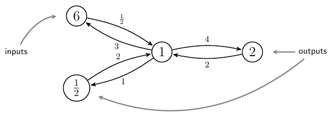
Here’s an example:
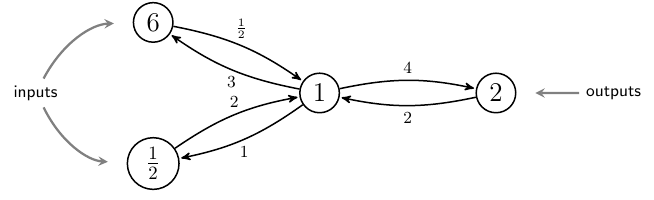
The detailed balanced Markov process itself consists of a finite set of states together with a finite set of edges between them, with each state labelled by an equilibrium population and each edge labelled by a rate constant
These populations and rate constants are required to obey an equation called the ‘detailed balance condition’. This equation means that in equilibrium, the flow from to equal the flow from to Do you see how it works in this example?
To get an ‘open’ detailed balanced Markov process, some states are designated as inputs or outputs. In general each state may be specified as both an input and an output, or as inputs and outputs multiple times. See how that’s happening in this example? It may seem weird, but it makes things work better.
People usually say Markov processes are all about how probabilities flow from one state to another. But we work with un-normalized probabilities, which we call ‘populations’, rather than probabilities that must sum to 1. The reason is that in an open Markov process, probability is not conserved: it can flow in or out at the inputs and outputs. We allow it to flow both in and out at both the input states and the output states.
Our most fundamental result is that there’s a category where a morphism is an open detailed balanced Markov process. We think of it as a morphism from its inputs to its outputs.
We compose morphisms in by identifying the output states of one open detailed balanced Markov process with the input states of another. The populations of identified states must match. For example, we may compose this morphism :
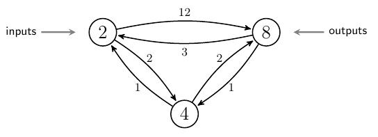
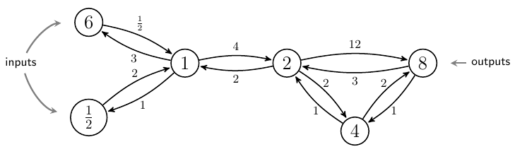
with the previously shown morphism to get this morphism :
And here’s our second most fundamental result: the category is actually a dagger compact category. This lets us do other stuff with open Markov processes. An important one is ‘tensoring’, which lets us take two open Markov processes like and above and set them side by side, giving :
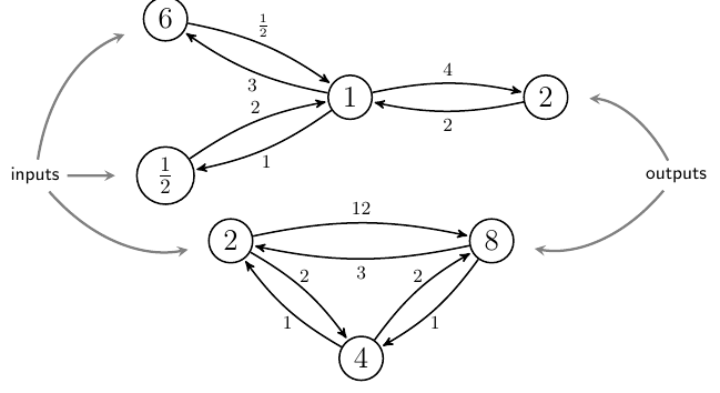
The compactness is also important. This means we can take some inputs of an open Markov process and turn them into outputs, or vice versa. For example, using the compactness of we can get this open Markov process from :
In fact all the categories in our paper are dagger compact categories, and all our functors preserve this structure. Dagger compact categories are a well-known framework for describing systems with inputs and outputs, so this is good.
The analogy to electrical circuits
In a detailed balanced Markov process, population can flow along edges. In the detailed balanced equilibrium, without any flow of population from outside, the flow along from state to state will be matched by the flow back from to The populations need to take specific values for this to occur.
In an electrical circuit made of linear resistors, charge can flow along wires. In equilibrium, without any driving voltage from outside, the current along each wire will be zero. The potentials will be equal at every node.
This sets up an analogy between detailed balanced continuous-time Markov chains and electrical circuits made of linear resistors! I love analogy charts, so this makes me very happy:
| Circuits | Detailed balanced Markov processes |
| potential | population |
| current | flow |
| conductance | rate constant |
| power | dissipation |
This analogy is already well known. Schnakenberg used it in his book Thermodynamic Network Analysis of Biological Systems. So, our main goal is to formalize and exploit it. This analogy extends from systems in equilibrium to the more interesting case of nonequilibrium steady states, which are the main topic of our paper.
Earlier, Brendan and I introduced a way to ‘black box’ a circuit and define the relation it determines between potential-current pairs at the input and output terminals. This relation describes the circuit’s external behavior as seen by an observer who can only perform measurements at the terminals.
An important fact is that black boxing is ‘compositional’: if one builds a circuit from smaller pieces, the external behavior of the whole circuit can be determined from the external behaviors of the pieces. For category theorists, this means that black boxing is a functor!
Our new paper with Blake develops a similar ‘black box functor’ for detailed balanced Markov processes, and relates it to the earlier one for circuits.
When you black box a detailed balanced Markov process, you get the relation between population–flow pairs at the terminals. (By the ‘flow at a terminal’, we more precisely mean the net population outflow.) This relation holds not only in equilibrium, but also in any nonequilibrium steady state. Thus, black boxing an open detailed balanced Markov process gives its steady state dynamics as seen by an observer who can only measure populations and flows at the terminals.
The principle of minimum dissipation
At least since the work of Prigogine, it’s been widely accepted that a large class of systems minimize entropy production in a nonequilibrium steady state. But people still fight about the the precise boundary of this class of systems, and even the meaning of this ‘principle of minimum entropy production’.
For detailed balanced open Markov processes, we show that a quantity we call the ‘dissipation’ is minimized in any steady state. This is a quadratic function of the populations and flows, analogous to the power dissipation of a circuit made of resistors. We make no claim that this quadratic function actually deserves to be called ‘entropy production’. Indeed, Schnakenberg has convincingly argued that they are only approximately equal.
But still, the ‘dissipation’ function is very natural and useful—and Prigogine’s so-called ‘entropy production’ is also a quadratic function.
Black boxing
I’ve already mentioned the category where a morphism is an open detailed balanced Markov process. But our paper needs two more categories to tell its story! There’s the category of circuits, and the category of linear relations.
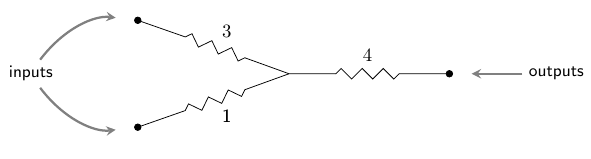
A morphism in the category is an open electrical circuit made of resistors: that is, a graph with each edge labelled by a ‘conductance’ together with specified input and output nodes:
A morphism in the category is a linear relation between finite-dimensional real vector spaces and This is nothing but a linear subspace Just as relations generalize functions, linear relations generalize linear functions!
In our previous paper, Brendan and I introduced these two categories and a functor between them, the ‘black box functor’:
The idea is that any circuit determines a linear relation between the potentials and net current flows at the inputs and outputs. This relation describes the behavior of a circuit of resistors as seen from outside.
Our new paper introduces a black box functor for detailed balanced Markov processes:
We draw this functor as a white box merely to distinguish it from the other black box functor. The functor maps any detailed balanced Markov process to the linear relation obeyed by populations and flows at the inputs and outputs in a steady state. In short, it describes the steady state behavior of the Markov process ‘as seen from outside’.
How do we manage to black box detailed balanced Markov processes? We do it using the analogy with circuits!
The analogy becomes a functor
Every analogy wants to be a functor. So, we make the analogy between detailed balanced Markov processes and circuits precise by turning it into a functor:
This functor converts any open detailed balanced Markov process into an open electrical circuit made of resistors. This circuit is carefully chosen to reflect the steady-state behavior of the Markov process. Its underlying graph is the same as that of the Markov process. So, the ‘states’ of the Markov process are the same as the ‘nodes’ of the circuit.
Both the equilibrium populations at states of the Markov process and the rate constants labelling edges of the Markov process are used to compute the conductances of edges of this circuit. In the simple case where the Markov process has exactly one edge from any state to any state the rule is this:
where:
- is the equilibrium population of the th state of the Markov process,
- is the rate constant for the edge from the th state to the th state of the Markov process, and
- is the conductance (that is, the reciprocal of the resistance) of the wire from the th node to the th node of the resulting circuit.
The detailed balance condition for Markov processes says precisely that the matrix is symmetric! This is just right for an electrical circuit made of resistors, since it means that the resistance of the wire from node to node equals the resistance of the same wire in the reverse direction, from node to node
A triangle of functors
If you paid careful attention, you’ll have noticed that I’ve described a triangle of functors:
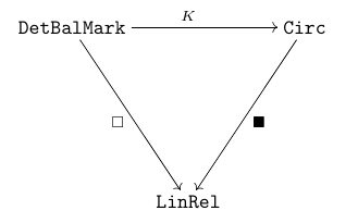
And if you’ve got the tao of category theory flowing in your veins, you’ll be wondering if this diagram commutes.
In fact, this triangle of functors does not commute! However, a general lesson of category theory is that we should only expect diagrams of functors to commute up to natural isomorphism, and this is what happens here:
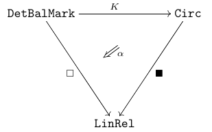
The natural transformation ‘corrects’ the black box functor for resistors to give the one for detailed balanced Markov processes.
The functors and are actually equal on objects. An object in is a finite set with each element labelled a positive populations Both functors map this object to the vector space For the functor we think of this as a space of population-flow pairs. For the functor we think of it as a space of potential-current pairs. The natural transformation then gives a linear relation
in fact an isomorphism of vector spaces, which converts potential-current pairs into population-flow pairs in a manner that depends on the I’ll skip the formula; it’s in the paper.
But here’s the key point. The naturality of actually allows us to reduce the problem of computing the functor to the problem of computing Suppose
is any morphism in The object is some finite set labelled by populations and is some finite set labelled by populations Then the naturality of means that this square commutes:
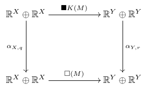
Since and are isomorphisms, we can solve for the functor as follows:
This equation has a clear intuitive meaning! It says that to compute the behavior of a detailed balanced Markov process, namely we convert it into a circuit made of resistors and compute the behavior of that, namely This is not equal to the behavior of the Markov process, but we can compute that behavior by converting the input populations and flows into potentials and currents, feeding them into our circuit, and then converting the outputs back into populations and flows.
What we really did
So that’s a sketch of what we did, and I hope you ask questions if it’s not clear. But I also hope you read our paper! Here’s what we actually do in there. After an introduction and summary of results:
- Section 3 defines open Markov processes and the open master equation.
- Section 4 introduces detailed balance for open Markov processes.
- Section 5 recalls the principle of minimum power for open circuits made of linear resistors, and explains how to black box them.
- Section 6 introduces the principle of minimum dissipation for open detailed balanced Markov processes, and describes how to black box these.
- Section 7 states the analogy between circuits and detailed balanced Markov processes in a formal way.
- Section 8 describes how to compose open Markov processes, making them into the morphisms of a category.
- Section 9 does the same for detailed balanced Markov processes.
- Section 10 describes the ‘black box functor’ that sends any open detailed balanced Markov process to the linear relation describing its external behavior, and recalls the similar functor for circuits.
- Section 11 makes the analogy between between open detailed balanced Markov processes and open circuits even more formal, by making it into a functor. We prove that together with the two black box functors, this forms a triangle that commutes up to natural isomorphism.
- Section 12 is about geometric aspects of this theory. We show that linear relations in the image of these black box functors are Lagrangian relations between symplectic vector spaces. We also show that the master equation can be seen as a gradient flow equation.
- Section 13 is a summary of what we have learned.
Finally, Appendix A is a quick tutorial on decorated cospans. This is a key mathematical tool in our work, developed by Brendan in an earlier paper.
Re: A Compositional Framework for Markov Processes
You lost me here. I’m looking at your example and I think I see how the detailed balance condition holds. On the right, for instance, we have flowing to the right and flowing to the left, which are equal.
Is it correct that the detailed balance condition implies that the populations are in equilibrium? Since at node there is the same amount flowing out to as flowing in from , for every individually.
Now none of this seems to have anything to do with choosing some states to call “input” and some to call “output”. Okay, you can choose some nodes and give them labels. But what is this “probability” thing? The only thing I can think of for it to mean is to sum up the populations and divide each of them by the total, so that in your example the total is , and the populations would get normalized to probabilities of . But dividing all the populations by the same number doesn’t affect the detailed balance condition or the fact that they are in equilibrium, does it? So what does it mean to say that probability is not conserved?
(By the way,
\leadstois apparently not supported in iTeX, but I think you can use\rightsquigarrow.)