On the Magnitude Function of Domains in Euclidean Space, I
Posted by Simon Willerton
.")
guest post by Heiko Gimperlein and Magnus Goffeng.
The magnitude of a metric space was born, nearly ten years ago, on this blog, although it went by the name of cardinality back then. There has been much development since (for instance, see Tom Leinster and Mark Meckes’ survey of what was known in 2016). Basic geometric questions about magnitude, however, remain open even for compact subsets of : Tom Leinster and Simon Willerton suggested that magnitude could be computed from intrinsic volumes, and the algebraic origin of magnitude created hopes for an inclusion-exclusion principle.
In this sequence of three posts we would like to discuss our recent article, which is about asymptotic geometric content in the magnitude function and also how it relates to scattering theory.
For “nice” compact domains in we prove an asymptotic variant of Leinster and Willerton’s conjecture, as well as an asymptotic inclusion-exclusion principle. Starting from ideas by Juan Antonio Barceló and Tony Carbery, our approach connects the magnitude function with ideas from spectral geometry, heat kernels and the Atiyah-Singer index theorem.
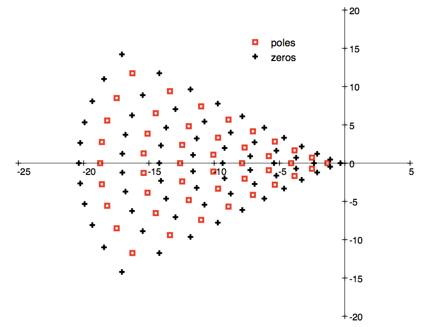
We will also address the location of the poles in the complex plane of the magnitude function. For example, here is a plot of the poles and zeros of the magnitude function of the -dimensional ball.
We thank Simon for inviting us to write this post and also for his paper on the magnitude of odd balls as the computations in it rescued us from some tedious combinatorics.
The plan for the three café posts is as follows:
State the recent results on the asymptotic behaviour as a metric space is scaled up and on the meromorphic extension of the magnitude function.
Discuss the proof in the toy case of a compact domain and indicate how it generalizes to arbitrary odd dimension.
Consider the relationship of the methods to geometric analysis and potential ramifications; also state some open problems that could be interesting.
Asymptotic results
As you may recall, the magnitude of a finite subset is easy to define: let be a function which satisfies
Such a function is called a weighting. Then the magnitude is defined as the sum of the weights:
For a compact subset of , Mark Meckes shows that all reasonable definitions of magnitude are equal to what you get by taking the supremum of the magnitudes of all finite subsets of :
Unfortunately, few explicit computations of the magnitude for a compact subset of are known.
Instead of the magnitude of an individual set , it proves fruitful to study the magnitude of dilates of , for . Here the dilate means the space with the metric scaled by a factor of . We can vary and this gives rise to the magnitude function of :
Tom and Simon conjectured a relation between the magnitude function of and its intrinsic volumes . The intrinsic volumes of subsets of generalize notions such as volume, surface area and Euler characteristic, with and .
Convex Magnitude Conjecture. Suppose is compact and convex, then the magnitude function is a polynomial whose coefficients involve the intrinsic volumes:
where is the -th intrinsic volume of and the volume of the -dimensional ball.
The conjecture was disproved by Barceló and Carbery (see also this post). They computed the magnitude function of the -dimensional ball to be the rational function In particular, the magnitude function is not even a polynomial for . Also, the coefficient of in the asymptotic expansion of as does not agree with the conjecture.
Nevertheless, for any smooth, compact domain in odd-dimensional Euclidean space, (in other words, the closure of an open bounded subset with smooth boundary), for , our main result shows that a modified form of the conjecture holds asymptotically as .
Theorem A. Suppose and that is a smooth domain.
There exists an asymptotic expansion of the magnitude function: with coefficients for .
The first three coefficients are given by where is the mean curvature of . (The coefficient was computed by Barceló and Carbery.) If is convex, these coefficients are proportional to the intrinsic volumes , and respectively.
For , the coefficient is determined by the second fundamental form and covariant derivative of : is an integral over of a universal polynomial in the entries of , . The total number of covariant derivatives appearing in each term of the polynomial is .
The previous part implies an asymptotic inclusion-exclusion principle: if , and are smooth, compact domains, faster than for all .
If you’re not familiar with the second fundamental form, you should think of it as the container for curvature information of the boundary relative to the ambient Euclidean space. Since Euclidean space is flat, any curvature invariant of the boundary (satisfying reasonable symmetry conditions) will only depend on the second fundamental form and its derivatives.
Note that part 4 of the theorem does not imply that an asymptotic inclusion-exclusion principle holds for all and , even if and are smooth, since the intersection usually is not smooth. In fact, it seems unlikely that an asymptotic inclusion-exclusion principle holds for general and without imposing curvature conditions, for example by means of assuming convexity of and .
The key idea of the short proof relates the computation of the magnitude to classical techniques from geometric and semiclassical analysis, applied to a reformulated problem already studied by Meckes and by Barceló and Carbery. Meckes proved that the magnitude can be computed from the solution to a partial differential equation in the exterior domain with prescribed values in . A careful analysis by Barceló and Carbery refined Meckes’ results and expressed the magnitude by means of the solution to a boundary value problem. We refer to this boundary value problem as the “Barceló-Carbery boundary value problem” below.
Meromorphic extension of the magnitude function
Intriguingly, we find that the magnitude function extends meromorphically to complex values of the scaling factor . The meromorphic extension was noted by Tom for finite metric spaces and was observed in all previously known examples.
Theorem B. Suppose and that is a smooth domain.
The magnitude function admits a meromorphic continuation to the complex plane.
The poles of are generalized scattering resonances, and each sector with contains at most finitely many of them (all of them outside ).
The ordinary notion of scattering resonances comes from studying waves scattering at a compact obstacle . A scattering resonance is a pole of the meromorphic extension of the solution operator to the Helmholtz equation on , with suitable boundary conditions. These resonances determine the long-time behaviour of solutions to the wave equation and are well studied in geometric analysis as well as throughout physics. The Barceló-Carbery boundary value problem is a higher order version of this problem and studies solutions to outside . In dimension (i.e. ), the Barceló-Carbery problem coincides with the Helmholtz problem, and the poles of the magnitude function are indeed scattering resonances. As in scattering theory, one might hope to find detailed structure in the location of the poles. A plot of the poles and zeros in case of the -dimensional ball is given at the top of the post.
The second part of this theorem is sharp. In fact, the poles do not need to lie in any half plane. Using the techniques of Barceló and Carbery we observe that the magnitude function of the 3-dimensional spherical shell is not rational and contains an infinite discrete sequence of poles which approaches the curve as . Here’s a plot of the poles of with .
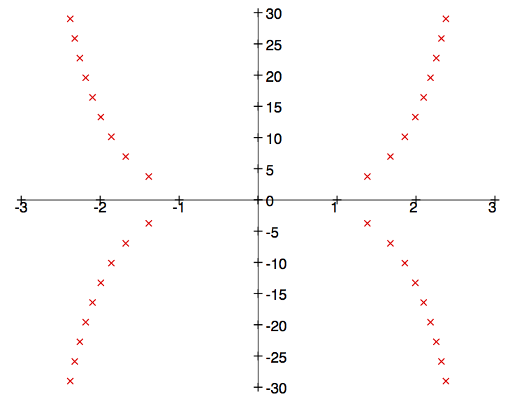
The magnitude function of is given by
[EDIT: The above formula has been corrected, following comments below.]
Our techniques extend to compact domains with a boundary, as long as is large enough. In this case, the asymptotic inclusion-exclusion principle takes the form that faster than for an .
Re: On the Magnitude Function of Domains in Euclidean Space, I.
Very interesting stuff! The question that leaps out to me is “Do you know anything about ?” The obvious guess would be something proportional to the total scalar curvature of , which is for convex . However, if memory serves me right, that is the integral of the second symmetric polynomial in the eigenvalues of the second fundamental form, so doesn’t involve the derivative of the second fundamental form, so your theorem seems to be indicating that it possibly isn’t that.