Turing Categories
Posted by John Baez
.")
guest post by Georgios Bakirtzis and Christian Williams
We continue the Applied Category Theory Seminar with a discussion of the paper Introduction to Turing Categories by Hofstra and Cockett. Thank you to Jonathan Gallagher for all the great help in teaching our group, and to Daniel Cicala and Jules Hedges for running this seminar.
Introduction
Turing categories enable the categorical study of computability theory, and thereby abstract and generalize the classical theory of computable functions on the natural numbers.
A Turing category is a category equipped with:
- cartesian products – to pair (the codes of) data and programs,
- a notion of partiality – to represent programs (morphisms) which do not necessarily halt,
- and a Turing object – to represent the “codes” of all programs.
The Turing object acts as a weak exponential for all pairs of objects in the category. While this is impossible in most “set-theoretical” categories, it is natural in computer science, because primitive formal languages—the “machine code” of the higher languages—are untyped (really one-typed).
For example, the untyped -calculus is represented by a reflexive object in a cartesian closed category, i.e. an object equipped with an embedding which sends a term to its action induced by application, and a retraction which sends an endo-hom term to the lambda term . The morphism is a Turing morphism, meaning that every morphism has a “code” such that
Turing categories are closely connected with partial combinatory algebras, magma objects with a certain form of “computational completeness”. The paradigmatic example is the “SK combinator calculus”, a variable-free representation of the calculus.
Turing categories and partial combinatory algebras (PCAs) are in a certain sense equivalent, which constitutes the main result of this work and justifies the notion of Turing category. (This is made into a precise equivalence of categories between relative PCAs and Turing categories over a fixed base category in the paper Categorical Simulations.)
Our purpose is to introduce the reader to some basic ideas in computability, and demonstrate how they can be expressed categorically.
Computability Theory
In the early 1900s, we focused intently on determining “what can we prove (with formal systems)?”, or analogously, “what can we compute (with computers)?”. This simple question inspired great advances in logic, mathematics, and computer science, and motivated their mutual development and deepening interconnection.
Three main perspectives emerged independently in order to answer this question:
- Alan Turing thought about “hardware”, with Turing machines;
- Alonzo Church thought about “software”, with the -calculus; and
- Kurt Gödel thought about logic, with general recursive functions.
The Church-Turing thesis states that these are equivalent notions of computation: a function is Turing computable iff can be written as a closed -term, iff is general recursive. This has led computer scientists to believe that the concept of computability is accurately characterized by these three equivalent notions.
Stephen Kleene, a student of Church, developed and unified these ideas in his study of “metamathematics”, focusing on the perspective of partial recursive functions (Introduction to Metamathematics – S.C. Kleene), which are equivalent to Gödel’s.
We can generate the class of partial recursive functions from basic functions and operators, and utilize the idea of Gödel numbering to consider the natural numbers both as the space of all data and all programs. The two main theorems which characterize an effective enumeration of all such functions—the Universality and Parameter theorems described below—are the original motivation for the definition of Turing categories.
Recursive Functions
Computability is humbly rooted in simple arithmetic. Using only three kinds of primitive functions, we can build up all computable functions, the partial recursive functions:
The set of primitive recursive functions, , is generated by two operators. First, we of course need composition:
Second, to derive real computational power we need the eponymous recursion:
This can be understood as a “for loop”— represents the initial parameters, is the counter, and describes a successive evaluation of the accumulated values—these are combined into the function :
Now we have enough to do arithmetic, and we’re off. For example, we can define addition: numbers are sequences of successors, and adding is simply a process of peeling the ’s off of one number and appending them to the other, until the former reaches 0:
As a simple demonstration:
Of course, not all computations actually halt. We can use a diagonalization argument to show that not all Turing-computable functions are primitive recursive. To complete the equivalence, the more general partial recursive functions are given by adding a minimization operator, which inputs a -ary function and outputs a -ary function, which searches for a minimal zero in the first coordinate of , and returns only if one exists:
This allows for “unbounded minimization of safe predicates”, to check the consistency of rules on infinitary data structures. For example, with this operator we can explicitly construct a universal Turing machine. The outputs of are certainly partial in general, because we can construct a predicate whose minimal zero would decide the halting problem.
All Turing-computable functions are represented by partial recursive functions, translating the complexity of Turing machines to a unified mathematical perspective of functions of natural numbers.
Gödel Numbering
Upon first hearing the Church-Turing thesis, one may ask “why do we only care about functions of natural numbers?” By the simple idea of Gödel numbering, we need only consider (the partial recursive subset of) the hom to think about the big questions of computability.
Kurt Gödel proved that a formal language capable of expressing arithmetic cannot be both consistent, meaning it does not deduce a contradiction, and complete, meaning every sentence in the language can be either proven or disproven. The method of proof is remarkably simple: as a language uses a countable set of symbols, operations, and relations, we can enumerate all terms in the language. We can then use this enumeration to create self-referential sentences which must be independent of the system.
The idea is to use the fundamental theorem of arithmetic. Finite lists of natural numbers can be represented faithfully as single natural numbers, using an encoding with prime powers: order the primes , and define the embedding
This can be applied recursively, to represent lists of lists of numbers, giving encoding functions enc for any depth and length of nested lists. The decoding, dec, is repeated factorization, forming a tree of primes. For example,
We can then enumerate the partial recursive functions: because they are generated by three basic functions and three basic operators, we can represent them as lists of natural numbers by the following recursive encoding “#”:
Then, a partial recursive function gives a list of lists, which can be encoded with Gödel numbering. For example,
So why do we want to enumerate all partial recursive functions? In contrast to the incompleteness theorems, this gives the theory of computability a very positive kind of self-reference, in the form of two theorems which characterize a “good” enumeration of partial recursive functions—this “good” means “effective” in a technical sense, namely that the kinds of operations one performs on functions, such as composition, can be computed on the level of codes.
Kleene’s Recursion Theorems
There is an enumeration of partial recursive functions , such that the following theorems hold.
Universality: The functions are partial recursive: .
Parameter: There are total recursive functions such that
The first says is a “universal computer”—we have partial for each arity, which takes (the code of) a program and (the code of) input data, and computes (the code of) the result. The second says this computer has generalized currying—there are total for each arity, which transforms -ary universal programs into -ary ones, by taking the first arguments and returning the code of another program.
This is a remarkable fact—imagine having a computer which comes preloaded with every conceivable program, and one simply inputs the number of the program, and the number of the data. Furthermore, if one does not know which program to use, one can determine even that one step at a time.
Turing categories are meant to provide a minimal setting in which these two theorems hold. The Universality Theorem describes the universal property of the Turing object/morphism pair, and the Parameter Theorem describes the fact that the factorizations of the -ary functions are determined by that of the unary ones, via the Turing morphism.
Restriction Categories
We have already discussed that a notion of partiality is necessary to model computation because not all computations halt at all inputs. This notion is concrete captured through the notion of partial functions. Partiality can be categorically described through restriction categories.
Formally, a restriction category is a category endowed with a combinator , sending
such that the following axioms are satisfied.
The first axiom states that precomposing with the domain of a map does not change or otherwise restrict the original. The second axiom states that restricting two functions behaves similarly to intersection in the sense that they commute. The third axiom states that taking the intersection of two domains is the same as taking either map and restricting it to the domain of the other map. The fourth axiom states that restricting a map in some other domain means that you restrict it on some other composite.
Some examples of restriction categories are:
If , then is total. Note that all monics are total. The total maps form a subcategory , which is of interest in the accompanying paper Total Maps of Turing Categories by Hofstra, Cockett, and Hrubeš. If , then is a domain of definition. For any Denote by the set of domains of definition of . For these examples:
Enrichment and Cartesian Structure
The notion of restriction entails a partial order on homsets—given , define Intuitively this means that the domain of is contained in the domain of . In the enrichment, forms a meet semilattice.
Accordingly, to define the cartesian structure we need to weaken the terminal object and product to the poset-enriched case.
Partial Terminal Object. Once we have partial maps, the terminal object acts like a “domain classifier”. Rather than having a unique map, we have a natural bijection For partial recursive functions over , we have precisely the recursively enumerable subsets. The partial terminal object satisfies the weaker universal property that given a domain and a map , the domain of the composite with any domain of is contained in .
The restriction terminal object, , is then describing the case when there is a unique total map such that . Furthermore, for each this family of maps must have to make the following diagram commute.

Partial Product. The partial product has the property that maps into the product, , which has the domain contained in that of both and . This is to account for the case in which computing and simultaneously might produce a result that either does not halt in or . Therefore, the domain of needs to be the intersection of the corresponding domains of and .

Splitting Idempotents
Turing categories are essentially meant to describe collections that can be computed by the maps of the category. This can be expressed with idempotent splitting. For example, in the “Turing category of computable maps on ”, explained later, a restriction idempotent is a recursively enumerable set. Therefore the splitting of , if it exists, makes this subset explicit as an object of the category. Hence, the idempotent completion of yields the category whose objects are all recursively enumerable sets of natural numbers. This will imply that these categories of computable maps are determined uniquely up to Morita equivalence.
There is, however, a big difference between split restriction categories and general restriction categories. In the former, all domains are “out in the open”, rather than “hiding” as idempotents on some object. If we completely understood the idempotent completion of , we would know all recursively enumerable subsets of ; one could argue that the study of computability would be complete. However, Turing categories are meant to abstract away from the natural numbers, in order to distinguish what is essential about computation, and remove anything about arithmetic that might be contingent.
Turing Categories
Turing categories provide an abstract framework for computability: a “category with partiality” equipped with a “universal computer”, whose programs and codes thereof constitute the objects of interest.
Let be a cartesian restriction category, and let . A morphism admits a -index when there exists such that the following commutes.
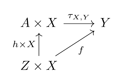
The -index can be thought of as an evaluation function and as the function . When every admits such an evaluation; that is -index, then is universal. If the object does this for any then is a Turing category and is a Turing object.
Given such a Turing category, , an applicative family for the Turing object is a family of maps , where , range over all objects in . An applicative family for is universal if for every , we have that is universal. In such a case is a Turing structure on . We can then think of a Turing structure on as a pair .
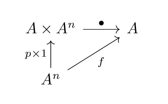
We can further express the universality of the Turing object in by taking every object of is a retract of , by taking the -index for .

This extends to all finite powers , which indicates two important points about the Turing object:
- The cardinality of the elements of , is either one or infinite; and
- There is an internal pairing operation , which is a section.
The latter morphism generalizes and abstracts the Gödel pairing .
So given such a universal object and a Turing structure , it is natural to wonder if a universal self-application map is special. It is indeed, and it is called a Turing morphism . Such a map, plus the universal property of , is in fact enough to reconstruct the entire Turing structure of .
The classic example is Kleene application . In general it can be thought of as a “universal Turing machine” that takes in a program (a Turing machine) and a datum, and computes the result.
This Turing morphism is the heart of the whole structure—we can construct all other universal applications by where pairs and retractions on and respectively.
To verify that is a universal application, consider the following commutative diagram, which shows that all subsets can be represented as formal objects and all computable functions, like , can be computed by representing them in .
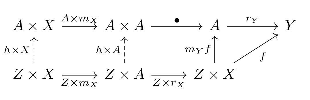
The important idea is that a Turing object represents the collection of (codes of) all programs in some formal system; the universal applicative family is a method of encoding, and the Turing morphism is the universal program which implements all others. The innovation of Turing categories is that they abstract away from , and can therefore describe programs which are not explicitly set-theoretical (not necessarily extensional, only intensional).
The axioms of a Turing structure correspond precisely to the Universality and Parameter theorems. This fact culminates in the Recognition Theorem: a cartesian restriction category is a Turing category iff there is an object of which every object is a retract, and for which there exists a Turing morphism .
Partial Combinatory Algebras
From the Recognition Theorem, we know that Turing categories are essentially generated by a single object equipped with a universal binary application. We can alternatively take the internal view, starting with a magma object in a cartesian restriction category , and consider maps which are “computable” with respect to . These maps form a category, and indeed a Turing category, iff is combinatory complete—essentially meaning that is expressive enough to represent the (partial) lambda calculus. First, we should understand combinators.
Combinatory Logic
The practice of variable binding is subtle: when a computation uses a set of symbols as variables, one must distinguish between bound and free variables—the former being placeholders, and the latter being data. In formal languages, preserving this distinction requires conditions of the semantic rules, which can add baggage to otherwise simple systems. In the -calculus, beta reduction precludes “variable capture”—accidentally substituting free into bound, e.g.: One must rename the bound variables of and so they are distinct from variables in both terms:
This problem was originally confronted by Moses Schonfinkel in the 1920s, who created a theory of combinators—primitive units of computation defined only by function application. Lambda terms can be translated into combinators by a process of abstraction elimination, which does away with variables completely. This can be understood by observing that we only need to handle the three basic things that occur within -abstraction: variables, application, and further abstraction. These are represented by the fundamental combinators and :
We can then define a recursive translation of terms:
For example, . This translation preserves exactly the way this term acts in the calculus. For more information, see To Mock a Mockingbird, and Eliminating Binders for Easier Operational Semantics.
Applicative Systems and Computable Maps
Let be a cartesian restriction category, and let be a magma object, a.k.a. an applicative system, in . A guiding example is Kleene application, . While we care about those which intuitively “act as universal Turing machines”, these are in fact a far more general concept. will be seen to generate a “category of computations”.
Comp(A)
A morphism is -, or simply computable, when there exists a total point , meaning has total domain, which provides the “code” for (like the -index):
This code picks out a program, i.e. an element of the universal Turing machine, which implements the function by application. When , we also require that is total. A morphism is computable if all components are, and a morphism is computable if its domain is (as a map ).
By weakening this diagram from commuting to being filled by a restriction 2-cell, i.e. , we generalize from computability to the realizability of , meaning that can be implemented or “realized” by restricting the code-application composite to the domain of , even if the former is defined more generally.
Of course in defining a morphism, we intend to form a category. With this general definition of computability, however, categorical structure does not come for free—for -computable morphisms to include identities and to be closed under composition, needs to have the right structure. This structure is directly connected to combinatory logic.
Let by the sub- (cartesian restriction) category of generated by all total points and application. These morphisms are called -polynomial morphisms. This essentially represents “all computations that knows how to do”. We should like that these are all computable, i.e. there exists codes for all of these “computations”. An applicative system is combinatory complete if every polynomial morphism is computable.
When is this true? Precisely when has the combinators S and K; that is, the following morphisms are -computable.
Let’s think about why this is true. As in the original use of combinators, we give a translation from -polynomial morphisms to composites of , application, and cartesian structure. This suffices because the generators of , the total points , are computable; then the polynomial construction essentially makes all possible application trees of these codes—and this is exactly what and do.
So, we define a partial combinatory algebra (PCA) to be an applicative system which is combinatory complete. We can now prove the simple categorical characterization of this completeness:
Theorem: For an applicative system in a cartesian restriction category , the following are equivalent:
is combinatory complete.
-computable morphisms form a cartesian restriction category.
(The forward direction: computable is a special case of being polynomial. The backward direction: the code of is the code of .)
What about the restriction structure? That is, given computable how do we know that is computable? This is actually given by the combinator :

i.e., .
Pairing a function with and projecting onto the first component gives the subdomain of on which the function is defined, and this operation is computable by the existence of the code . These combinators are humble but very useful.
Hence, we have a direct equivalence between the classical notion of combinatory completeness and the general, abstract computability concept of cartesian restriction category. (Like many “generalizations” in abstract mathematics, it’s really more an extension than generalization, because we still depend on the original idea of combinatory completeness; but “grounding” the latter by seeing it as a natural structure in a fully abstract setting demonstrates essential understanding, and connects the concept to the rest of category theory and computer science.)
Examples
The most important example of a category of computable maps is , of natural numbers and Kleene application.
Another example is the (partial) lambda calculus, modelled by a reflexive object as mentioned in the introduction.
One can generalize these examples by adding further expressive power such as oracles, or by considering “basic recursive function theories” which are sets of functions satisfying the Universality and Parameter theorems.
Structure Theorem
Now, for the unsurprising and important conclusion: given a PCA , the computable maps form not only a cartesian restriction category, but a Turing category. The application is the Turing morphism, and the codes are the indices. The pairing operator pair: is represented by the lambda term , and projections fst,snd: are given by , . One can check that these satisfy fst pair = and snd pair = . We then have (pair, fst, snd gives the product as a retract of , and this extends to . Hence, is a Turing object, and is a Turing category.
Thus, we have the main theorem:
Structure Theorem
Let be a cartesian restriction category with applicative system .
When is a in , then is a Turing category with Turing object .
If is a Turing category and is a Turing object, then is a in and is Morita-equivalent to .
Conclusion
We learned some about the roots of computability theory, and discussed how Turing categories abstract these ideas, using the guiding example of natural numbers and partial recursive functions. Every Turing category arises from a partial combinatory algebra, in particular the natural numbers with Kleene application. Conversely, every partial combinatory algebra determines a Turing category, establishing the latter and raising the former into more general abstraction. Turing categories remain an active area of research, and our group looks forward to studying and contributing to this work.
Re: Turing Categories
Thank you for the introductory post on this subject, it looks interesting!
I was just wondering about the remark that you made about Turing objects:
If I understand it correctly, there is the universal Turing morphism , and it is a retraction with a section . And there is a section . I guess internal pairing is the later operation, because the former one is an evaluation map?