Octonions and the Standard Model (Part 6)
Posted by John Baez
.")
One of the most interesting functions on the exceptional Jordan algebra is the determinant. The linear transformations that preserve this form the exceptional Lie group . And today I’ll show you how to compute this determinant in terms of 10-dimensional spacetime geometry: that is, scalars, vectors and spinors in 10d Minkowski spacetime.
The exceptional Jordan algebra consists of self-adjoint matrices of octonions. The diagonal entries are forced to be their own conjugate, hence real:
Thus, is 27-dimensional.
is a Jordan algebra with product
where at right we’re just doing ordinary matrix multiplication. The group of linear transformations that preserve this product is 52-dimensional and it’s called : it’s one of the five exceptional compact simple groups, and everyone should learn to love it.
is not just coincidentally connected to the exceptional Jordan algebra. It’s deeply connected. For example, its smallest nontrivial representation is 26-dimensional! Why 26 and not 27? Because it acts on in a way that preserves the identity, and also the inner product
so it preserves the 26-dimensional space of elements orthogonal to the identity: the traceless self-adjoint self-adjoint matrices of octonions, .
But the exceptional Jordan algebra also has another nice structure: the determinant. You might worry that the determinant of a matrix of octonions is ill-defined, since the octonions are noncommutative and nonassociative. And that’s true in general. But there’s a nice way to define it for a self-adjoint matrix of octonions:
See? This is beautiful. It’s even better when you know that , and that is invariant under cyclic permutations of , so we could rewrite this formula in a number of ways and get the same thing.
The transformations in preserve this determinant, but many others do too. There is a 78-dimensional group of linear transformations of that preserve the determinant. It’s called , it’s a noncompact exceptional simple Lie group, and again you should learn to love it. It’s deeply connected to : for example, this space is its smallest nontrivial representation.
Actually this group is called , since has a number of different noncompact real forms, and this particular one has as its maximal compact subgroup, so it has
extra noncompact directions. Indeed, as a manifold — though not as a Lie group — we have
But I don’t plan to talk about any other real form of anytime soon, so for now I’ll just call this one .
By the way, note that 26, 52 and 78 are all multiples of 26. This is part of the spooky numerology that you learn when you get into exceptional Lie groups. That you see above is really : the 26-dimensional space of traceless elements of .
But I’m getting ahead of myself!
Last time I explained how the exceptional Jordan algebra could be chopped into three parts, which correspond to scalars, vectors and left-handed spinors in 10d Minkowski spacetime. This time I’ll say how the determinant can be expressed in terms of these parts.
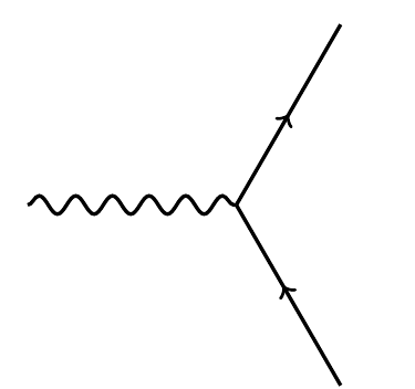
In the end we’ll have a formula for the determinant in terms of various operations involving scalars, vectors and spinors in 10d spacetime. The most exciting of these describes how a spin-1/2 fermion (described by a spinor of one handedness) can absorb a spin-1 boson (described by a vector) and turn into another spin-1/2 fermion (described by a spinor of the other handedness):
All these operations will be invariant under the group . As an immediate consequence we get an inclusion
This has a nice meaning! As we saw last time, is 10d Minkowski spacetime. The group acts as symmetries. We can think of as an ‘exceptional’ 27-dimensional spacetime containing 10d Minkowski spacetime, with symmetry group . A point in this larger spacetime consists of a point in 10d Minkowski spacetime — that is, a vector — together with a scalar and a left-handed spinor. While acts on vectors, only its double cover acts on spinors. So we get an inclusion of , not , in .
I hope to continue developing the theme of as a funny sort of ‘exceptional spacetime’ later. But we need to start by understanding the main structures on . For this I want to express the determinant on in terms of invariant operations on scalars, vectors and spinors in 10d Minkowski spacetime.
Intertwining operators
We might as well get our money’s worth and let be any normed division algebra or . We’ll let stand for its dimension: 1, 2, 4, or 8. Last time I described representations of on
scalars:
vectors:
right-handed spinors
left-handed spinors
Now let’s describe some equivariant maps that relate these representations. Another name for an equivariant map between group representations is an ‘intertwining operator’— that’s what all my old books say, but it seems to be a bit old-fashioned: some of my students have never even heard of it!
By the way, a lot of these maps exist quite generally for scalars, vectors, and spinors in Minkowski spacetimes of any dimension — so this stuff is good to learn if you care about physics at all. But we get nice formulas for them using division algebras in Minkowski spacetimes of dimensions and .
Here they are:
1) An invariant pairing, our friend the Minkowski metric
given by
where the tilde stands for trace reversal:
which, as we saw last time, has the geometrical meaning of time reversal.
2) An invariant pairing between right- and left-handed spinors:
given by
where the dagger stands for conjugate transpose. Here I’m thinking of as column vectors, so is a row vector and the product is an element of . This pairing is nondegenerate, so
as representations of .
3) An action of vectors on right-handed spinors that turns them into left-handed spinors:
given by
where in we’re multiplying a matrix and a column vector.
4) An action of vectors on left-handed spinors that turns them into right-handed spinors:
given by
In physics, maps 3) and 4) are used to describe how a spin-1/2 particle can absorb a gauge boson and turn into another spin-1/2 particle:
We saw last time that they also give rise to the action of the spin group on spinors of either handedness.
These maps give others using duality: we can turn inputs into outputs, or vice versa, by taking their duals. For example, our map also gives a map , but using our invariant pairings we can re-express this as a map . We can get a map in the same way. It’s worth having formulas for these maps:
5) An equivariant map that turns two left-handed spinors into a vector:
given by
Here we are multiplying column vectors by row vectors and getting matrices, and when we add those up the end result is self-adjoint.
6) An equivariant map that turns two right-handed spinors into a vector:
given by
where the impressively long tilde stands for trace reversal.
To see proofs that maps 1)–6) are intertwining operators, see Section 3 here:
- John C. Baez, John Huerta, Division algebras and supersymmetry I, in Superstrings, Geometry, Topology, and C-algebras, eds. R. Doran, G. Friedman and J. Rosenberg, Proc. Symp. Pure Math. 81, AMS, Providence, 2010, pp. 65–80.
I’m trying to make these blog articles self-contained, but you can just pop over there for the details.
The determinant
As we’ve seen, the determinant of
is
But we can break up into its scalar, vector and spinor parts:
where
Then we have:
Theorem 8. For any we have
Proof. Start with the definition
You can see the determinant of the block
hiding in this expression, and as I mentioned last time, , so
Thus to prove the theorem we just need to show
So, let’s compute the left-hand side! We have
and thus
Multiplying the damned matrices and taking the real part of their trace, we get
which is close to what we want. The first and last terms in the parentheses are already real and match what we’re shooting for, so we just need to show
For this we use two normed division algebras facts: the cyclic property of the real part, and its invariance under conjugation:
So we’re done! █
Some spinoffs
It follows from the theorem that the group of determinant-preserving transformations of contains . In the case we care about most, this gives an inclusion of Lie groups
and thus an inclusion of Lie algebras
Now the dimension of is 78 — or so I’ve claimed without proof. The dimension of is the triangular number . Since
we could look for an interesting 33-dimensional space whose direct sum with gives — as vector spaces, not as Lie algebras. And indeed we have one, since and are 16-dimensional. It’s !
And in fact, there’s a nice way to put a Lie bracket on to get an isomorphism of Lie algebras
By ‘nice’, I mean it’s geometrically well-motivated. So we get a description of in terms of 10-dimensional spacetime geometry!
We can also try this game with division algebras that are less glamorous than the octonions. It’s worth doing, even if we only care about the exceptional case, just to get some analogues that are easier to understand. If we take , the same argument winds up showing that
We then count:
We should try to copy what worked before. In this case as vector spaces, so is 5-dimensional! And indeed we get a nice isomorphism
where again ‘nice’ means that it’s motivated by the geometry.
If we use , we get
We then count:
In this case as vector spaces, so is just 9-dimensional as a real vector space. So close and yet so far! But it turns out that everything is okay: we have a nice isomorphism
Finally, we can move to the quaternionic case and try the same trick. We get
The determinant of a quaternionic matrix is a tricky thing, but it’s real valued, so while has real dimension , it has a Lie subgroup of dimension just one less, namely .
We then count:
In this case and are 8-dimensional, so has dimension 20. So I’m willing to guess… but I’m not completely sure… that we get a nice isomorphism
I should check this someday.
- Part 1. How to define octonion multiplication using complex scalars and vectors, much as quaternion multiplication can be defined using real scalars and vectors. This description requires singling out a specific unit imaginary octonion, and it shows that octonion multiplication is invariant under .
- Part 2. A more polished way to think about octonion multiplication in terms of complex scalars and vectors, and a similar-looking way to describe it using the cross product in 7 dimensions.
- Part 3. How a lepton and a quark fit together into an octonion — at least if we only consider them as representations of , the gauge group of the strong force. Proof that the symmetries of the octonions fixing an imaginary octonion form precisely the group .
- Part 4. Introducing the exceptional Jordan algebra : the self-adjoint octonionic matrices. A result of Dubois-Violette and Todorov: the symmetries of the exceptional Jordan algebra preserving their splitting into complex scalar and vector parts and preserving a copy of the adjoint octonionic matrices form precisely the Standard Model gauge group.
- Part 5. How to think of self-adjoint octonionic matrices as vectors in 10d Minkowski spacetime, and pairs of octonions as left- or right-handed spinors.
- Part 6. The linear transformations of the exceptional Jordan algebra that preserve the determinant form the exceptional Lie group . How to compute this determinant in terms of 10-dimensional spacetime geometry: that is, scalars, vectors and left-handed spinors in 10d Minkowski spacetime.
- Part 7. How to describe the Lie group using 10-dimensional spacetime geometry. This group is built from the double cover of the Lorentz group, left-handed and right-handed spinors, and scalars in 10d Minkowski spacetime.
- Part 8. A geometrical way to see how is connected to 10d spacetime, based on the octonionic projective plane.
- Part 9. Duality in projective plane geometry, and how it lets us break the Lie group into the Lorentz group, left-handed and right-handed spinors, and scalars in 10d Minkowski spacetime.
- Part 10. Jordan algebras, their symmetry groups, their invariant structures — and how they connect quantum mechanics, special relativity and projective geometry.
- Part 11. Particle physics on the spacetime given by the exceptional Jordan algebra: a summary of work with Greg Egan and John Huerta.
- Part 12. The bioctonionic projective plane and its connections to algebra, geometry and physics.
Re: Octonions and the Standard Model (Part 6)
for literature references, isn’t called an Albert Algebra?