The n-Category Café

A Brief Introduction to Linear Logic

Before getting to the definition of LDCs, it is helpful to build intuition around the linear setting for which they are named. Note that this section is adapted from Priyaa Srinivasan’s 2021 thesis.

• P.V. Srinivasan. Dagger Linear Logic and Categorical Quantum Mechanics. PhD thesis, Department of Computer Science, University of Calgary, 2021.

Linear logic was introduced by Girard in 1987 as a logic for resource manipulation. Linear logic can be viewed as a refinement of other logic systems in that it joins the dualities of classical logic with the constructive properties of intuitionistic logic. Operationally, this means linear logic isn’t about expanding “truths” but manipulating resources that can’t be duplicated or thrown away at will.

Take, for example, the following statements, $p$ and $q$: $$\begin{aligned} &{\color{#9B26B6}p} : \text{to spend a dollar} \\ &{\color{#9B26B6}q} : \text{to buy an apple} \end{aligned}$$

The compound statement “$p \Rightarrow q$” means that if a dollar is spent then an apple can be bought. One can have either a dollar or an apple at a given time but not both. Once the dollar is spent, $p$ is no longer true until another dollar obtained. Hence, the linear sensitivity of this logic is illustrated by a series of resource transformations.

The fragment of linear logic we are concerned with is known as multiplicative linear logic (MLL), which has connectives ($\otimes$, 1, $\oplus$, $\bot$). These connectives correspond to conjunction/disjunction as well as “and/or” from classical logic. The statement $A \otimes B$ (read as “A times B” or “A tensor B”), for example, allows one the means to access both resources at the same time (e.g., if $r$ is an orange, then “$p \Rightarrow q \otimes r$” means both an apple and an orange are available to purchase at the same time). The formula 1 is the multiplicative truth of this fragment ($A \otimes 1 = 1 \otimes A = A$).

$\oplus$ (read as “par”), on the other hand, is the dual to $\otimes$ and acts as the multiplicative disjunction. (One should beware the notation for par introduced by Cockett and Seely conflicts with Girard’s original notation; we will stick with Cockett and Seely’s version for this post.) In this case, $\bot$ is the dual to 1 (i.e., false). Linear logic also has an additive fragment and exponential operators (which allow linear logic to deal with non-linearity), but we won’t be mentioning them in detail here as our focus is on the binary operations of the multiplicative fragment.

A proof of a statement in linear logic may be regarded as a series of resource transformations. More generally, the proof theory used to define linear logic is derived from a Gentzen-style sequent calculus. A formal proof in this calculus is a sequence of so-called “sequents” that explicitly record dependencies line-by-line (i.e., each sequent is derivable from sequents appearing earlier in the sequence using logical or structural inference rules).

In the sequent calculus of linear logic, each line of a proof is written in the general form of $\Gamma \vdash \Delta$. The sequent places a context (thought of as a collection of resources) on each side of the turnstile, thereby separating the assumptions on the left-hand side from the propositions on the right-hand side. In this way, linear logic is often considered as a two-sided logic. We offer a few simple examples to illustrate the nature of this logic system and highlight key points that led to the development of categorical semantics and LDCs based on this sequent calculus.

Left introduction rule for $\otimes$

Consider a string or sequence of propositions, where $\Gamma$ and $\Delta$ are collections of resources.

$$\Gamma_1, A, B, \Gamma_2 \vdash \Delta$$

The structural rules are for rewriting either the left-hand side or right-hand side of the sequent. For example, one can combine the terms on the left-hand side by tensoring them.

In the notation above, the top line can be thought of as the premise and the bottom line the conclusion. In this case, the left introduction rule is an inference rule that introduces a logical connective ($\otimes$) in the conclusion of the sequent. By introducing tensor on the left-hand side of the turnstile, the conclusion means one needs both resources $A$ and $B$ to produce $\Delta$.

Right introduction rule for $\oplus$

The same introduction rules can be done with par, but for par, the collection of resources must be combined on the right-hand side of the turnstile (i.e., when left of the turnstile, the sequence is conjunctive; when right of the turnstile, the sequence is disjunctive).

There are also elimination rules, which are dual to the introduction rules, but we will not be elaborating on them here.

Cut rule

The cut rule allows formulae to be “cut out” and the respective derivation joined. In the example below, the formula $B$ is highlighted to show where the cut will take place.

With this inference rule, one can combine sequents based on their shared boundary, such as in the example above, where the formula $B$ is “cut out” and used to stick together the constituent premises to form a composite conclusion. Category theorists may recognize the cut rule, as it is just like composition. This begs the question if there is a categorical structure for this…

Linearly Distributive Categories

Definition of LDCs

To recap, we have covered the basics of the multiplicative fragment of linear logic (or MLL), we gave its resource-theoretic interpretation, and we briefly touched upon its Gentzen-style sequent calculus. But while sequent calculus is a versatile framework for MLL, as Priyaa Srinivasan writes in her 2021 thesis, “[p]roofs in sequent calculus often contain extraneous details due [to] the sequential nature of the calculus.” For instance, when applying rules to a sequent, an order of application needs to be specified, even if the rules are independent. This begs for an equivalent but notationally cleaner formulation of MLL, which is precisely what we will explore in this section. Specifically, we will explore linearly distributive categories (LDCs), which were first outlined in Cockett and Seely’s 1997 paper under the name weakly distributive categories. The incredible discovery of Cockett and Seely’s paper is that it recognizes that the fundamental property of linear logic is a kind-of “linearization” of the traditional distributivity of product over sum now called a linear distributor. However, we will not prove this fact here, directing the interested reader to the first section on polycategories and Theorem 2.1 in Cockett and Seely’s 1997 paper. Instead, we will take the fact that LDCs model MLL on faith, and only focus on exploring LDCs, so without further ado, we define LDCs.

A linearly distributive category (or a weakly distributive category) is a category $\mathbb{X}$ with two monoidal structures $$(\mathbb{X}, \otimes, \top, a_\otimes, u_\otimes^L, u_\otimes^R) \quad \text{and} \quad (\mathbb{X}, \oplus, \bot, a_\oplus, u_\oplus^L, u_\oplus^R),$$ where $\otimes$ is a monoidal tensor called “times” with a monoidal unit $\top \in \operatorname{Ob}{\mathbb{X}}$ called “top” or “true,” and $\oplus$ is a monoidal tensor called “par” with a monoidal unit $\bot \in \operatorname{Ob}{\mathbb{X}}$ called “bottom” or “false.” Since the times $\otimes$ is monoidal, it is equipped with the three familiar natural isomorphisms $$\begin{aligned} &a_\otimes : (A \otimes B) \otimes C \rightarrow A \otimes (B \otimes C) \\ &u_\otimes^L : \top \otimes A \rightarrow A \\ &u_\otimes^R : A \otimes \top \rightarrow A, \end{aligned}$$ called the times associator, the left times unitor, and the right times unitor, respectively, which (of course) satisfy the monoidal triangle and pentagon equations. Likewise, as the par $\oplus$ is also monoidal, we have another set of three natural isomorphisms $$\begin{aligned} &a_\oplus : (A \oplus B) \oplus C \rightarrow A \oplus (B \oplus C) \\ &u_\oplus^L : \bot \oplus A \rightarrow A \\ &u_\oplus^R : A \oplus \bot \rightarrow A \end{aligned}$$ called the par associator, the left par unitor, and the right par unitor, respectively.

However, there is nothing particularly interesting about two independent monoidal structures in the same category; what makes LDCs interesting is the interaction between these two monoidal structures, which consists of so-called linear distributors. Specifically, the times $\otimes$ and par $\oplus$ are linked by the two natural transformations $$\begin{aligned} &\delta_L^L : A \otimes (B \oplus C) \rightarrow (A \otimes B) \oplus C \\ &\delta_R^R : (B \oplus C) \otimes A \rightarrow B \oplus (C \otimes A), \end{aligned}$$ which are called the left and right linear distributors, respectively, and these distributors are required to satisfy a couple dozen coherence conditions, as specified in section 2 of Cockett and Seely’s 1997 paper. While these maps have “distributor” in their name, that is pretty much the end of $\delta_L^L$ and $\delta_R^R$’s relation to distributive categories. Distributivity does not guarantee the existence of left and right distributors, and as Cockett and Seely found, the two tensors of a distributive category form an LDC if and only if the category is a preorder, making LDCs and distributive categories practically orthogonal constructs. The important thing to note is that, unlike for the traditional distributor, the object $A$ can only “attach” itself to one of the arguments of the sum $\oplus$. To give the resource-theoretic intuition behind this, one can imagine that the object $A$ represents a waiter, Alice, at a restaurant, and objects $B$ and $C$ represent two seated guests, Bob and Carol, at different tables. Alice can assign herself to serve either Bob (i.e., perform $\delta_L^L$) or Carol (i.e., perform $\delta_R^R$), but not both simultaneously. It is also important to note that these linear distributors do not in general represent an equality and are not invertible. So continuing our analogy, once Alice has assigned herself to either Bob or Carol, Alice cannot go back to a state where she can make that choice again, i.e., a state where she can switch the guest she is assigned to.

In addition to the aforementioned two linear distributors, the LDC $\mathbb{X}$ can also have the two permuting linear distributors $$\begin{aligned} &\delta_R^L : A \otimes (B \oplus C) \rightarrow B \oplus (A \otimes C) \\ &\delta_L^R : (B \oplus C) \otimes A \rightarrow (B \otimes A) \oplus C. \end{aligned}$$ When our LDC has the $\delta_R^L$ and $\delta_L^R$ natural transformations, it is called a non-planar LDC. Note that if the times $\otimes$ and par $\oplus$ of the LDC $\mathbb{X}$ are symmetric, we can create the permuting linear distributors $\delta_R^L$ and $\delta_L^R$ from the traditional linear distributors $\delta_L^L$ and $\delta_R^R$ with the times $\otimes$ and par $\oplus$ braidings (denoted by $s_\otimes$ and $s_\oplus$, respectively), making the LDC $\mathbb{X}$ automatically a non-planar LDC.

Graphical Calculus for LDCs

Note that this subsection and its figures are adapted from Cockett, Comfort, and Srinivasan’s 2021 paper on dagger linear logic.

• J.R.B. Cockett, C. Comfort, and P.V. Srinivasan, “Dagger linear logic for categorical quantum mechanics,” Logical Methods in Computer Science Volume 17, Issue 4, 10.46298/lmcs-17(4:8)2021, 2021.

Now that we described the basics of LDCs, you at this point may be asking what, then, makes LDCs so notationally special. Certainly, there is nothing particularly striking in the definition: an LDC is just two intertwined monoidal structures. But, it is precisely this structure that creates a rich graphical calculus (similar to monoidal graphical calculus), which provides us a versatile framework to perform entirely graphical manipulations on problems in the multiplicative fragment of linear logic. We direct the reader to Blute, Cockett, Seely, and Trimble’s 1996 paper Natural deduction and coherence for weakly distributive categories for a complete and rigorous discussion on the graphical calculus. Nevertheless, we will briefly discuss this graphical calculus here to give the reader some familiarity with the subject.

To start off, in the graphical calculus for LDCs, wires represent objects, circles represent morphisms, composition is done by stacking morphisms vertically, and we read diagrams from top to bottom. Recall that in general, sequents in linear logic (or morphisms in the LDC) go from tensored formulae (or objects in the LDC) to “par”ed formulae, so the input wires of a morphism are tensored (with $\otimes$), and the output wires are “par”ed (with $\oplus$). For instance, $f : A \otimes B \to C \oplus D$ is denoted graphically by

The comonoid-like shape at the top of the diagram represents $\otimes$-elimination, and what it denotes is the process of taking a tensor product like $A \otimes B$ and splitting it up, with $A$ exiting through one wire and $B$ exiting through the other, allowing us to hypothetically operate on $A$ and $B$ independently. The monoid-like shape at the bottom of the diagram, on the other hand, represents $\oplus$-introduction, and it denotes taking two objects, say $A$ and $B$, and “par”ing them, resulting in the combined object $A \oplus B$ exiting the process. In addition to these, we have an analogous $\oplus$-elimination, which is denoted graphically , and $\otimes$-introduction, which is denoted graphically by . 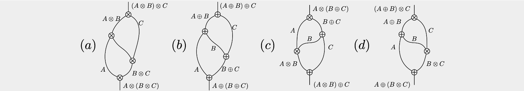With $\otimes$-elimination, $\oplus$-introduction, $\oplus$-elimination, and $\otimes$-introduction, we denote graphically the $\otimes$-associator $a_\otimes$, the $\oplus$-associator $a_\oplus$, the left linear distributor $\delta_L^L$, and the right linear distributor $\delta_R^R$ as

The final building blocks of this graphical calculus are those for the unitors, which are drawn as

The diagram in (a) is called the left $\top$-introduction, the diagram in (b) is called the left $\top$-elimination, the diagram in (c) is called the left $\bot$-introduction, and the diagram in (d) is called the left $\bot$-elimination. There is an analogous set of four diagrams for the right $\otimes$-unitor and the right $\oplus$-unitor which are just horizontal reflections of the four diagrams above.

Once a morphism is expressed as a circuit using the building blocks above, there are numerous graphical manipulations one can perform, just as in monoidal graphical calculus. We refer the reader to Blute, Cockett, Seely, and Trimble’s 1996 paper to see these graphical manipulations. However, it is very important to note that not every circuit that can be constructed from these building blocks represents a valid morphism in our LDC. To check if a circuit is valid, one needs to show that the entire circuit can be enclosed in a single “box” by successfully using the rules $(a_1)$-$(e_4)$ listed below:

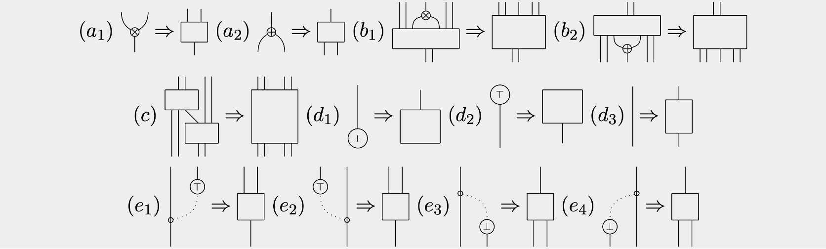
For example, applying the boxing algorithm to the left linear distributor $\delta_L^L$, we can see that the circuit can be encapsulated in one box, making it a valid circuit.

But the reverse circuit cannot be “boxed” because a $\otimes$-elimination cannot be absorbed by a box above it and $\oplus$-introduction cannot be absorbed by a box below it.

This shows us why the inverse of the left linear distributor $\delta_L^L$ is not in general possible, but it is important to note that this does not mean that there does not exist any LDC with an inverse to $\delta_L^L$. In the $\bot$-shifted tensor example below, $\delta_L^L = a_\otimes^{-1}$, which is invertible by definition.

LDC Example: The $\bot$-Shifted Tensor

Now that we have defined the LDC, let us explore a simple example of one. In this section, we explore the $\bot$-shifted tensor. To start off, we assume we are given a category $\mathbb{X}$ with a monoidal structure $(\mathbb{X}, \otimes, \top, a_\otimes, u_\otimes^L, u_\otimes^R)$ with a tensor inverse, which is an object $\bot\in\operatorname{Ob}{\mathbb{X}}$ such that there exists an object $\bot^{-1}\in\operatorname{Ob}{\mathbb{X}}$ and two isomorphisms $$s^L : \bot \otimes \bot^{-1} \to \top \quad \text{and} \quad s^R : \bot^{-1} \otimes \bot \to \top$$ such that the diagram below commutes.

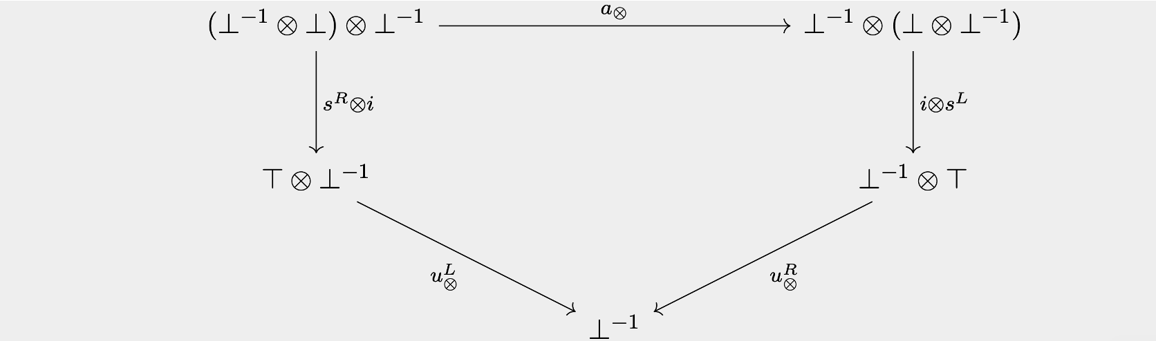
Note that at this point, we do not have the ingredients to declare that $\mathbb{X}$ is an LDC. Namely, we are missing a second monoidal structure (i.e., the par $\oplus$) and linear distributors (i.e., $\delta_L^L$ and $\delta_R^R$), so in order to show that $\mathbb{X}$ is an LDC, we need to construct the par and the linear distributors, which we are able to do with the tensor inverse $\bot^{-1}$ along with its corresponding isomorphisms $s^L$ and $s^R$.

We choose to define our par tensor $\oplus$ by $$X \oplus Y = X \otimes (\bot^{-1} \otimes Y),$$ and we will take $\bot$ to be the unit for the $\oplus$ tensor. This tensor we call the $\bot$-shifted tensor. We then define the associator $a_\oplus$, left unitor $u^L_\oplus$, and right unitor $u^R_\oplus$ for par $\oplus$ using the natural isomorphisms from the $\otimes$ monoidal structure and the tensor inverse’s isomorphisms $s^L$ and $s^R$, as shown below. (Note that the equalities below are of the natural transformations, not the objects.) $$\begin{aligned} &\qquad A \oplus \bot \xrightarrow{u_\oplus^R} A = A \otimes (\bot^{-1} \otimes \bot) \xrightarrow{i \otimes s^R} A \otimes \top \xrightarrow{u_\otimes^R} A \\ &\qquad \bot \oplus A \xrightarrow{u_\oplus^L} A = \bot \otimes (\bot^{-1} \otimes A) \xrightarrow{a_\otimes^{-1}} (\bot \otimes \bot^{-1}) \otimes A \xrightarrow{s^L \otimes i} \top \otimes A \xrightarrow{u_\otimes^L} A \\ &(A \oplus B) \oplus C \xrightarrow{a_\oplus} A \oplus (B \oplus C) = (A \otimes (\bot^{-1} \otimes B)) \otimes (\bot^{-1} \otimes C) \\ &\qquad\qquad\qquad\qquad\qquad\qquad\qquad\qquad\xrightarrow{a_\otimes ; i \otimes a_\otimes} A \otimes (\bot^{-1} \otimes (B \otimes (\bot^{-1} \otimes C))). \end{aligned}$$ Using the monoidal triangle and pentagon equations for $\otimes$ and the coherence diagram for the tensor inverse’s isomorphisms $s^L$ and $s^R$, we can show that our constructed structure $(\mathbb{X}, \oplus, \bot, a_\oplus, u_\oplus^L, u_\oplus^R)$ satisfies the monoidal triangle and pentagon equations, giving us a second monoidal structure. But are there linear distributors between these two monoidal structures? In fact, there do exist linear distributors for this category, and looking at the necessary domains and codomains, it is not too hard to see that they are just associators. We can define a left and a right linear distributor by $$\begin{aligned} &A \otimes (B \oplus C) \xrightarrow{\delta_L^L} (A \otimes B) \oplus C = A \otimes (B \otimes (\bot^{-1} \otimes C)) \xrightarrow{a_\otimes^{-1}} (A \otimes B) \otimes (\bot^{-1} \otimes C) \\ &(B \oplus C) \otimes A \xrightarrow{\delta_R^R} B \oplus (C \otimes A) = (B \otimes (\bot^{-1} \otimes C)) \otimes A \xrightarrow{a_\otimes;i \otimes a_\otimes} B \otimes (\bot^{-1} \otimes (C \otimes A)). \end{aligned}$$ These maps satisfy all the LDC coherence conditions, making any monoidal category with a tensor inverse an LDC!

$\ast$-Autonomous Categories

The Negative Object Map $(-)^\bot$

Now that we have covered a categorical framework for the multiplicative fragment of linear logic via LDCs, we are interested in adding into this framework a notion of negation, and this is precisely what we will explore in this section. In this brief section, we will study $\ast$-autonomous categories, which provide a categorical presentation of MLL with negation. But before we treat that, we will begin by just adding two negation functions on the objects of an LDC, so without further ado:

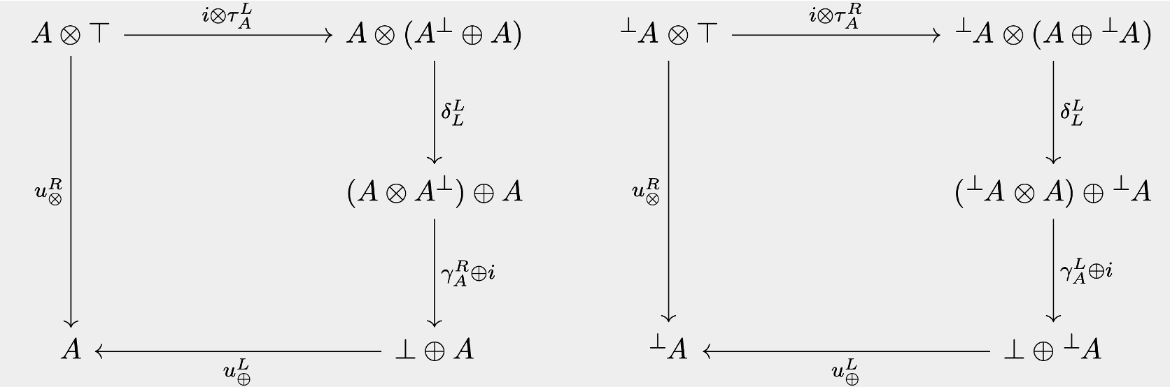
A linearly distributive category $\mathbb{X}$ with negation is a regular LDC with two functions on objects of $\mathbb{X}$, which we denote by $(-)^\bot$ and ${}^\bot(-)$, where we have the parameterized families of morphisms $$\begin{aligned} &\gamma_A^L : {}^\bot{A} \otimes A \rightarrow \bot \\ &\gamma_A^R : A \otimes A^\bot \rightarrow \bot \\ &\tau_A^L : \top \rightarrow A^\bot \oplus A \\ &\tau_A^R : \top \rightarrow A \oplus {}^\bot{A}. \end{aligned}$$ These morphisms must satisfy the coherence conditions $$\begin{aligned} &i \otimes \tau_A^L ; \delta_L^L ; \gamma_A^R \oplus i ; u_\oplus^L = u_\otimes^R \\ &\tau_A^R \otimes i ; \delta_R^R ; i \oplus \gamma_A^L ; u_\oplus^R = u_\otimes^L \\ &i \otimes \tau_A^R ; \delta_L^L ; \gamma_A^L \oplus i ; u_\oplus^L = u_\otimes^R \\ &\tau_A^L \otimes i ; \delta_R^R ; i \oplus \gamma_A^R ; u_\oplus^R = u_\otimes^L, \end{aligned}$$ where, for instance, the commutative diagrams for the first (left) and third (right) coherence conditions are

While reading this definition, you may have noticed something rather odd: nowhere in the definition of an LDC with negation do we require that $(-)^\bot$ and ${}^\bot(-)$ be functors. In fact, we do not even request that $(-)^\bot$ and ${}^\bot(-)$ act on morphisms at all; we only require that these maps act on objects. The reason for this is that an LDC with negation has sufficient structure to make $(-)^\bot$ and ${}^\bot(-)$ into functors without requiring this a priori. Specifically, if for any morphism $f : A \to B$ in $\mathbb{X}$, we define ${}^\bot f : {}^\bot{B} \to {}^\bot{A}$ by $$\begin{split} {}^\bot f &: {}^\bot{B} \xrightarrow{(u_\otimes^R)^{-1}} {}^\bot{B} \otimes \top \xrightarrow{i \otimes \tau_A^R} {}^\bot{B} \otimes (A \oplus {}^\bot{A}) \xrightarrow{i \otimes (f \oplus i)} {}^\bot{B} \otimes (B \oplus {}^\bot{A}) \\ &\qquad\quad \xrightarrow{\delta_L^L} ({}^\bot{B} \otimes B) \oplus {}^\bot{A} \xrightarrow{\gamma_B^L \oplus i} \bot \oplus {}^\bot{A} \xrightarrow{u_\oplus^L} {}^\bot{A}, \end{split}$$ then ${}^\bot(-)$ extends to a contravariant functor. A similar definition makes $(-)^\bot$ into a contravariant functor.

Now that we have an LDC with negation, let us better understand how this structure implements a notion of negation. The key lies in the four parameterized families of morphisms $\gamma_A^L$, $\gamma_A^R$, $\tau_A^L$, and $\tau_A^R$. To give intuition as to why this is the case, let us treat $(-)^\bot$ & ${}^\bot(-)$ as “not,” $\top$ as “true,” $\bot$ as “false,” $\otimes$ as “and,” and $\oplus$ as “or.” Then with this interpretation, $\gamma_A^L$ reads as “not $A$ and $A$ implies false,” $\gamma_A^R$ reads as “$A$ and not $A$ implies false,” $\tau_A^L$ reads as “true implies not $A$ or $A$,” and finally, $\tau_A^R$ reads as “true implies $A$ or not $A$,” implying that the morphisms $\gamma_A^L$ & $\gamma_A^R$ encode in our LDC a notion of “contradiction,” and the morphisms $\tau_A^L$ & $\tau_A^R$ encode “tertium non datur,” giving our LDC a notion of negation.

To continue our discussion of how our “LDC with negation” models logical negation, we need one formal property of LDCs with negation, which is that they have the following adjunctions. $$\begin{matrix} A \otimes - \dashv A^\bot \oplus - &&& {}^\bot{A} \otimes - \dashv A \oplus - \\ - \otimes B \dashv - \oplus {}^\bot{B} &&& - \otimes B^\bot \dashv - \oplus B \end{matrix}$$ The proof of this is not too hard, but we will only provide a sketch of the proof that $- \otimes B$ is left adjoint to $- \otimes {}^\bot{B}$ for brevity. To do this, we need to find a unit $\eta$ and counit $\varepsilon$ for the adjunction. In this case, the unit $\eta : A \to (A \otimes B) \oplus {}^\bot{B}$ is given by $$\eta : A \xrightarrow{(u^R_\otimes)^{-1}} A \otimes \top \xrightarrow{i \otimes \tau_B^R} A \otimes (B \oplus {}^\bot{B}) \xrightarrow{\delta_L^L} (A \otimes B) \oplus {}^\bot{B},$$ and the counit $\varepsilon : (A \oplus {}^\bot{B}) \otimes B \to A$ is given by $$\varepsilon : (A \oplus {}^\bot{B}) \otimes B \xrightarrow{\delta_R^R} A \oplus ({}^\bot{B} \otimes B) \xrightarrow{i \oplus \gamma_B^L} A \oplus \bot \xrightarrow{u_\oplus^R} A$$ for all $A \in \operatorname{Ob}{\mathbb{X}}$. Now that we have proposed a unit and counit for the adjunction, we need to show that they satisfy the triangle identity, but doing so necessitates a quite lengthy diagram chase, so we refer the reader to Lemma 4.2 in Cockett and Seely’s 1997 paper to see the commutative diagram that proves this.

The reason we mentioned this property of LDCs with negation is because these adjunctions give us the following bijections.

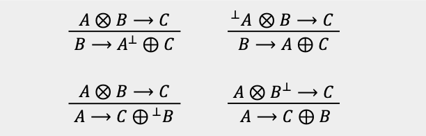
Continuing our intuition from before, we can interpret the top-left bijection as telling us that “$A$ and $B$ implies $C$” is equivalent (or more precisely, isomorphic) to “$B$ implies not $A$ or $C$,” which is exactly how we would expect negation to work in logic. Similarly, the top-right bijection tells us that “not $A$ and $B$ implies $C$” is equivalent to “$B$ implies $A$ or $C$,” which is again exactly what we would expect from negation in logic. And so on.

Definition and Graphical Calculus for $\ast$-Autonomous Categories

Now that we have encoded negation into our LDC, we will define an interesting type of LDC with negation: a case where we only need one negation map $(-)^\bot$. This type of LDC is called a symmetric linearly distributive category $\mathbb{X}$ with negation, which is a regular LDC where the $\otimes$ and $\oplus$ monoidal structures have symmetric braidings, which we denote by $s_\otimes$ and $s_\oplus$, respectively, such that the diagram below commutes.

In addition to the symmetric braidings $s_\otimes$ and $s_\oplus$, the symmetric LDC $\mathbb{X}$ with negation has a function $(-)^\bot$ defined on the objects of $\mathbb{X}$ along with the following morphisms for every object $A$: $$\begin{aligned} &\gamma_A^R : A \otimes A^\bot \to \bot \\ &\tau_A^R : \top \to A \oplus A^\bot. \end{aligned}$$ These induce the following families $$\begin{aligned} &\gamma_A^L : A^\bot \otimes A \to \bot \\ &\tau_A^L : \top \to A^\bot \oplus A, \end{aligned}$$ which together satisfy the following main coherence conditions $$\begin{aligned} &i \otimes \tau_A^L ; \delta_L^L ; \gamma_A^R \oplus i ; u_\oplus^L = u_\otimes^R \\ &i \otimes \tau_A^R ; \delta_L^L ; \gamma_A^L \oplus i ; u_\oplus^L = u_\otimes^R \end{aligned}$$ (as well as related coherence conditions that arise from fundamental symmetries of non-planar LDCs). It turns out (as is shown in Cockett and Seely’s 1997 paper) that a symmetric linearly distributive category with negation is completely equivalent to a $\ast$-autonomous category, giving us another axiomatization of $\ast$-autonomous category that is, in many instances, easier to prove. In the next section, we will give an example of a category that is $\ast$-autonomous, which we will prove by showing that it is a symmetric LDC with negation.

But before we continue on to that example, we will take a brief digression to look at the coherence conditions of the symmetric LDC with negation. On the face of it, these two coherence conditions look complicated and uninteresting. However, when we draw the equations in our graphical calculus for LDCs (suppressing units), we get a remarkable structure, which is shown below.

To the reader who is familiar with monoidal graphical calculus, you will instantly recognize these as the “snake” or “yanking” equations for compact closed monoidal categories, which allow curved lines in a diagram to be straightened. Hence, a symmetric LDC with negation (or a $\ast$-autonomous category) has a notion of yanking curved lines straight in the graphical calculus for LDCs. However, a $\ast$-autonomous category is not a compact closed monoidal category, and $\tau$ and $\gamma$ are not the same as the unit and counit of the dual for a compact closed monoidal category, as $\gamma$ maps to the monoidal unit of par $\oplus$ and $\tau$ maps from the monoidal unit of times $\otimes$, and these two monoidal units $\bot$ and $\top$ are not in general equal. This makes $\ast$-autonomous categories very interesting for studying infinite-dimensional quantum mechanics. To elaborate on the reason: the snake equations have been extensively used in finite-dimensional quantum mechanics, which can be modeled by a compact closed monoidal category FdHilb. Unfortunately, once you move from finite dimensions to infinite dimensions, the monoidal category Hilb is no longer compact closed. However, with a $\ast$-autonomous category, it becomes possible to create a notion of “yanking” equations straight without the category being compact closed, which is a promising feature for modeling infinite-dimensional quantum mechanics. This is still a very active area of research, and we direct the interested reader to Priyaa Srinivasan’s thesis for a comprehensive treatment on the topic.

$\ast$-Autonomous Categories Example: The Abelian Group

In the prior section, we introduced $\ast$-autonomous categories (well actually, we introduced the equivalent notion of symmetric LDCs with negation), so in this section we are going to explore an example of one: an abelian group. Let us consider an abelian group $(G, 0, +)$, where we choose at random one of the elements in $G$, which we denote by $a$. We can interpret this abelian group $(G, 0, +)$ as a symmetric monoidal category, where we take the objects of $G$ to be the objects of the category, we take $+$ to be the monoidal tensor, we take $0$ to be the monoidal unit, and we say there is a morphism $x$ to $y$ for $x, y \in G$ if and only if $x = y$ (which implies that all diagrams commute automatically by transitivity!). So, for example, because of this interpretation and the fact that $(G, 0, +)$ is an abelian group, we know our induced category has an associator, as $(x + y) + z = x + (y + z)$ for all $x,y,z \in G$; a left unitor, as $0 + x = x$ for all $x \in G$; a right unitor, as $x + 0 = x$ for all $x \in G$; and a symmetric braiding, as $x + y = y + x$ for all $x, y \in G$. The fact that the pentagon and triangle equations are satisfied is immediate via transitivity as we mentioned above, thereby justifying our earlier statement that our abelian group $(G, 0, +)$ is really just a symmetric monoidal category. In fact, it is a monoidal category with a tensor inverse $a$, but let us ignore that fact for the remaining discussion, as we want to work out this example from scratch.

We will take the $+$ monoidal structure to be the par monoidal structure for the LDC. But we still need to find a second monoidal structure for the times. Let us define $\bullet$ by $x \bullet y = x + y + (-a)$, where $-a$ is the inverse of $a$, and let us take $a$ to be its unit. Clearly, for all $x, y, z \in G$, $$\begin{aligned} a \bullet x &= a + x + (-a) = x + a + (-a) = x \\ x \bullet a &= x + a + (-a) = x \\ (x \bullet y) \bullet z &= [x + y + (-a)] + z + (-a) = x + [y + z + (-a)] + (-a) = x \bullet (y \bullet z) \\ x \bullet y &= x + y + (-a) = y + x + (-a) = y \bullet x, \end{aligned}$$ so our binary operator $\bullet$, with $a$ as its unit, has a left unitor, a right unitor, an associator, and a symmetric braiding, giving us our second symmetric monoidal structure, which we will take to be the times monoidal structure for the LDC.

Now, we need linear distributors. Since, for all $x, y, z \in G$, $$\begin{aligned} x \bullet (y + z) &= x + (y + z) + (-a) = [x + y + (-a)] + z = (x \bullet y) + z \\ (y + z) \bullet x & = (y + z) + x + (-a) = y + [z + x + (-a)] = y + (z \bullet x), \end{aligned}$$ our category has a left linear distributor and a right linear distributor. The coherences are immediately satisfied via transitivity, so our abelian group $(G, 0, +)$ with a designated invertible element $a$ is an LDC. Since our par $+$ and our times $\bullet$ have symmetric braidings, to show that our category is $\ast$-autonomous, all we need to show is that we have a map $(-)^\bot$ on objects such that there exists a “contradiction” map $\gamma_x^R : x \bullet x^\bot \to 0$ and a “tertium non datur” map $\tau_x^R : a \to x + x^\bot$ for all $x \in G$. Let us define $x^\bot = -x + a$, where $-x$ is the inverse of $x$, for all $x \in G$. Then, for all $x \in G$, $$\begin{aligned} x \bullet x^\bot &= x + [(-x) + a] + (-a) = x + (-x) + a + (-a) = 0 \\ a &= 0 + a = [x + (-x)] + a = x + [(-x) + a] = x + x^\bot, \end{aligned}$$ which implies that $\gamma_x^R$ and $\tau_x^R$ exist. Thus, the abelian group $(G, 0, +)$ is a $\ast$-autonomous category.