This afternoon’s first talk is by Masaki Tsukamoto, who’s giving an introduction to Gromov’s notion of mean dimension. I’ll paste in the abstract:
Mean dimension is a topological invariant of dynamical systems introduced by Gromov in 1999. It is a dynamical version of topological dimension. It evaluates the number of parameters per unit time for describing a given dynamical system. Gromov introduced this notion for the purpose of exploring a new direction of geometric analysis. Independently of this original motivation, Elon Lindenstrauss and Benjamin Weiss found deep applications of mean dimension in topological dynamics. I plan to survey some highlights of the mean dimension theory.
Tsukamoto works in dynamical systems and ergodic theory, and explained to us the idea of “dynamicalization”: take concepts and theorems in geometry, and find analogues in dynamical systems.
For example:
number of points topological entropy
pigeonhole principle symbolic coding
New example by Gromov: topological dimension mean dimension.
Slogan:
Mean dimension is the number of parameters per unit time for describing a dynamical system.
Plan for the talk:
- Topological entropy and symbolic dynamics
- Mean dimension and topological dynamics
- Mean dimension and geometric analysis
Topological entropy and symbolic dynamics
For now, a dynamical system is a compact metrizable space with a homeomorphism , or equivalently, a continuous -action. So then we can consider generalizing from to other groups.
For , define as the minimum number of open sets of diameter needed to cover . Now for , put
This is a metric. The topological entropy of is
Example Let be a finite set, and consider the full shift on the alphabet , which is the dynamical system defined by
Then we get
Generally, here’s a recipe for dynamicalization: given an invariant of spaces , define a dynamical version so that
We just did this for cardinality. What about the pigeonhole principle?
Some terminology. An embedding of dynamical systems is a topological embedding that commutes with and .
What obstructions are there to existence of dynamical embeddings? Write for the set of periodic points of period dividing . If embeds in then:
- for all .
A partial converse holds! A closed subset of is called a subshift if . The Krieger embedding theorem says that if and are finite sets and satisfies:
- ,
- for all ,
then embeds in . Note that can be much larger than !
This is the dynamical version of the pigeonhole principle, in the following version: a finite set embeds in a finite set iff . We’ve just changed the appropriate notion of size.
Mean dimension and topological dynamics
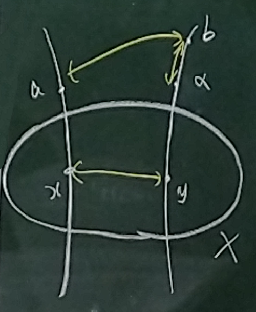
A continuous map of metric spaces is called an -embedding if each fibre has diameter . For compact , define (width dimension) as the minimum integer for which can be -embedded into an -dimensional simplicial complex.
The topological dimension of is
This is a topological invariant!
Theorem (Menger and Nöbeling) If then topologically embeds in .
Short digression: every compact metric space of topological dimension 1 can be topologically embedded into the Menger sponge (itself a subspace of ).
The dynamical embedding problem Consider the shift map on the Hilbert cube . When does a given dynamical system embed in ?
Periodic points again provide an obstruction. If does embed in then embeds in .
Allan Jaworski proved in his 1974 PhD thesis that if is a finite-dimensional system (i.e. ) and has no periodic point then embeds in . Then he left mathematics and became an artist.
What about infinite-dimensional systems? Joseph Auslander asked in 1988: can we embed every minimal dynamical system in in the shift of the Hilbert cube? Minimal means that every orbit is dense, e.g. an irrational rotation of the circle. (This is a topological analogue of ergodicity.) Minimality clearly precludes the existence of periodic points: it’s a strong version of there being no periodic points.
The answer came about a decade later. In 1999, Mikhail Gromov introduced mean dimension, defined by
Again, this is a topological invariant!
If is a nice space then
In this sense, mean dimension is the dynamicalization of topological dimension.
Earlier we had the slogan:
Mean dimension is the number of parameters per unit time for describing a dynamical system.
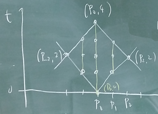
Here’s an informal (or maybe I mean formal?) explanation of the “per unit time” bit:
In particular,
But if embeds in then one easily shows that
So if then it doesn’t embed in the shift of the Hilbert cube! Lindenstrauss and Weiss found in 2000 that for any , there is some minimal dynamical system of mean dimension. IN particular, there is some minimal system not embeddable in the shift of the Hilbert cube.
Lindenstrauss proved a further result that if a minimal dynamical system has mean dimension smaller than then it embeds in the shift of . And, with the speaker Tsukamoto, he proved that this constnt 36 can’t be improved to 2 or less. Finally, Tsukamoto and Gutman proved that it can be improved to 2. So that completely settles that question.
Mean dimension and geometric analysis
The talk then went into more advanced material on Gromov’s original motivation, which was from geometry rather than symbolic dynamics. Gromov was interested in groups acting on manifolds , with a PDE on M and its space of solutions. I decided to concentrate on listening to this part rather than taking notes.
This was a really wonderful talk, with beautiful conceptual structure. I now think of dynamicalization as a cousin of categorification and feel irresistibly drawn to try to find something new to dynamicalize.
.")


Colloquium: Introduction to magnitude
There was a kind of pre-event yesterday, a colloquium for the Osaka University mathematics department which I gave:
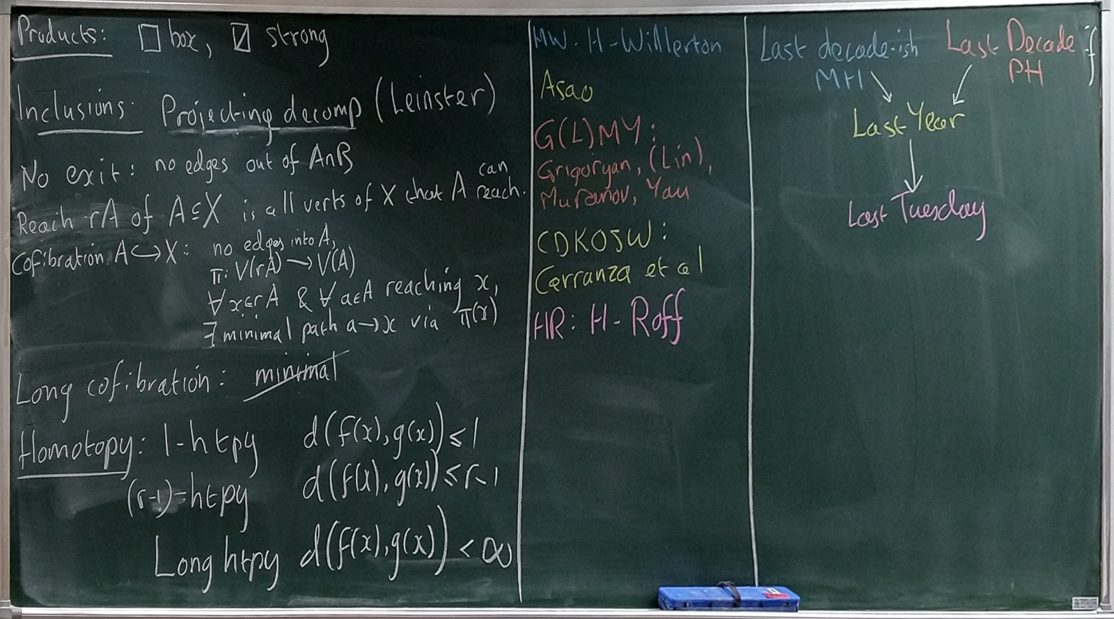
If you’ve seen me give a general talk on magnitude then many of the slides will be familiar to you. But I want to draw your attention to a new one (page 27), which is a summary of recent and current activity in magnitude homology and is meant to whet your appetite for some of the talks this week.
Here’s that slide in plain text, shorn of the photos of the people involved:
What’s happening in magnitude homology?
There is a relationship between magnitude homology and persistent homology — but they detect different information (Nina Otter; Simon Cho)
Applications of magnitude homology to the analysis of networks (Giuliamaria Menara)
A theory of magnitude cohomology (Richard Hepworth)
Connections between magnitude homology and path homology (Yasuhiko Asao)
A comprehensive spectral sequence approach that encompasses both magnitude homology and path homology (Yasuhiko Asao; Richard Hepworth and Emily Roff; also relevant is work of Kiyonori Gomi)
A concept of magnitude homotopy (Yu Tajima and Masahiko Yoshinaga)
New results on magnitude homology equivalence of subsets of , involving convex geometry (joint with Adrián Doña Mateo)
And lots more… find out this week!