Skip to the Main Content

Note:These pages make extensive use of the latest XHTML and CSS Standards. They ought to look great in any standards-compliant modern browser. Unfortunately, they will probably look horrible in older browsers, like Netscape 4.x and IE 4.x. Moreover, many posts use MathML, which is, currently only supported in Mozilla. My best suggestion (and you will thank me when surfing an ever-increasing number of sites on the web which have been crafted to use the new standards) is to upgrade to the latest version of your browser. If that's not possible, consider moving to the Standards-compliant and open-source Mozilla browser.

July 10, 2012

Morton and Vicary on the Categorified Heisenberg Algebra

Posted by John Baez

Wow! It’s here!

Back when I was working with Jeffrey Morton on categorifying the harmonic oscillator, I discovered to my surprise that there was another guy, a student of Chris Isham named Jamie Vicary, who was also categorifying the harmonic oscillator, using different but related ideas. Luckily, they started to collaborate… and they discovered some quite wonderful things.

In quantum mechanics, position times momentum does not equal momentum times position! This sounds weird, but it’s connected to a very simple fact. Suppose you have a box with some balls in it, and you have the magical ability to create and annihilate balls. Then there’s one more way to create a ball and then annihilate one, than to annihilate one and then create one.

Huh? Yes: if there are, say, 3 balls in the box to start with, there are 4 balls you can choose to annihilate after you’ve created one but only 3 before you create one.

In quantum mechanics, when you’re studying the harmonic oscillator, it’s good to think about operators that create and annhilate… not balls, but ‘quanta of energy’. The creation operator is called a a^\dagger and the annihilation operator is called aa, and the argument I just sketched can be used to show that

aa =a a+1 a a^\dagger = a^\dagger a + 1

It’s a wonderful fact that you can express the position qq and momentum pp of the oscillator in terms of these creation and annihilation operators:

q=a+a 2,p=aa 2i q = \frac{a + a^\dagger}{\sqrt{2}} , \qquad p = \frac{a - a^\dagger}{\sqrt{2} \, i}

So the fact that position and momentum don’t commute, but instead obey

pqqp=i p q - q p = -i

(in units where Planck’s constant is 1) can be seen as coming from the more intuitive fact that the annihilation and creation operators don’t commute, but instead obey

aa a a=1 a a^\dagger - a^\dagger a = 1

This insight, that funny facts about quantum mechanics are related to simple facts about balls in boxes, allows us to ‘categorify’ a chunk of quantum mechanics—including the Heisenberg algebra, which is the algebra generated by the position and momentum operators. Now is not the time to explain what that means. The important thing is that Mikhail Khovanov figured out a seemingly quite different way to categorify the same chunk of quantum mechanics, so there was a big puzzle about how his approach relates to the one I just described. Jeffrey Morton and Jamie Vicary have solved that puzzle.

The big spinoff is this. Khovanov’s approach showed that in categorified quantum mechanics, a bunch of new equations are true! These equations are ‘higher analogues’ of Heisenberg’s famous formula

pqqp=i p q - q p = -i

So, these new equations should be important! But they look very mysterious at first:

In fact, when I first saw them, it seemed as if Khovanov had just plucked them randomly from thin air! Of course he had not: they arose from the representation theory of symmetric groups. But their intuitive meaning was far from transparent.

Now Jeffrey and Jamie have shown how to get these equations just by thinking about balls in boxes. The equations in fact make perfect sense! See Section 2.8: Combinatorial Interpretation for details. Let me just get you started. We should replace the equation

a a+1=aa a^\dagger a + 1 = a a^\dagger

by an isomorphism

a a+1aa a^\dagger a + 1 \stackrel{\sim}{\Rightarrow} a a^\dagger

This provides a one-to-one correspondence between ‘ways to annihilate a ball and then create one… together with one more thing’ and ‘ways to create a ball and then annihilate it’. This isomorphism is built from two parts:

f:a aaa f: a^\dagger a \Rightarrow a a^\dagger

and g:1aa g: 1 \Rightarrow a a^\dagger

The thing I’m calling

f:a aaa f: a^\dagger a \Rightarrow a a^\dagger

says how every way to annihilate a ball (say the ball xx) and then create a different one (say yxy \ne x) gives a way to create one (namely yy) and then annihilate one (namely xx). The thing I’m calling

g:1aa g: 1 \Rightarrow a a^\dagger

says how there is one other way to create a ball and then annihilate one: namely, by annihilating the same ball we just created!

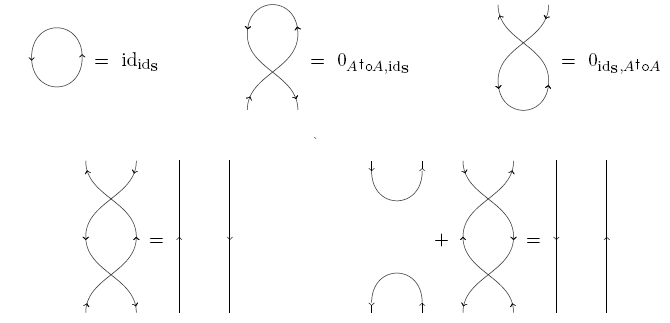
The five equations shown in the picture above are then a clever graphical way of describing basic facts about the morphisms ff and gg and two others which are a bit subtler to describe. These others, which deserve to be called

f :aa a af^\dagger: a a^\dagger \Rightarrow a^\dagger a

and

g :aa 1g^\dagger : a a^\dagger \Rightarrow 1

do not give functions that send one way to do things to another. Instead, they give relations. You can’t ‘turn around’ a function and get a function going the other way unless it’s invertible. But you can turn around a function and get a relation going the other way.

I’ve hit the limit on what I can explain without getting more serious and ruining the light-hearted, easy-going tone of this post. If you want details, I’d rather just let you read the paper!

But I’d like to say a few fancier things, just for the experts. In reality, what matters most for Jeffrey and Jamie are not sets and relations, but groupoids and spans of groupoids. Spans of groupoids allow you to ‘turn around’ a functor between groupoids. In our old work on categorifying quantum mechanics, Jeffrey and I used the bicategory of

  • groupoids,
  • spans of groupoids,
  • isomorphism classes of maps of spans of groupoids.

Recently Alex Hoffnung has shown this is a monoidal bicategory—in fact part of a monoidal tricategory if you don’t wimp out and take isomorphism classes at the 2-morphism level, as I just did. (Alex, to his credit, did not.) Mike Stay has gone further and shown it’s a compact closed symmetric monoidal bicategory.

As I said, spans of groupoids let you ‘turn around’ a functor between groupoids, like h:XYh: X \to Y and get something going the other way, which we denote with a dagger:

h :YXh^\dagger : Y \to X

This is how we construct the annihilation operator a a^\dagger starting from the creation operator aa in categorified quantum mechanics. But to define 2-morphisms like f f^\dagger and g g^\dagger above, Jeffrey and Jamie need to turn around maps of spans of groupoids. And to do this, we need spans of spans of groupoids. So they need a monoidal bicategory like this:

  • groupoids,
  • spans of groupoids,
  • isomorphism classes of spans of spans of groupoids.

They show that the equations in Khovanov’s categorified Heisenberg algebra follow from equations between 2-morphisms here… which have nice combinatorial interpretations in terms of balls in boxes!

It would be interesting to see what happens if we go even further. We don’t really need to stop at spans of spans. We could keep on going forever, as noted in the famous Monte Python song:

Span, span, span, span,
span, span, span, span…

If we went one notch further we could categorify our categorified Heisenberg algebra and get a 2-categorified Heisenberg algebra. We would find that the equations relating f,g,f f, g, f^\dagger and g g^\dagger became isomorphisms, and we could work out what equations those isomorphisms and their daggers satisfy!

The important thing is this: those equations are not something we get to choose, or make up. They are what they are, and they’re just sitting there waiting for us to discover them.

It could be that these higher equations are trivial for some reason. That would be interesting: it would mean that Khovanov’s categorified Heisenberg algebra is the end of the story, not the tip of an even deeper iceberg. Or, maybe these equations are nontrivial! That would be even more interesting!

Of course, there’s also a lot to think about without categorifying further. What if any physical meaning do the relations in the categorified Heisenberg algebra have? Can we actually do something like physics with some categorified version of quantum theory? Or is this stuff mainly good for understanding the representation of symmetric groups in a deeper way, using combinatorics? That would already be very interesting. And so on…

Posted at July 10, 2012 9:16 AM UTC

TrackBack URL for this Entry:   https://golem.ph.utexas.edu/cgi-bin/MT-3.0/dxy-tb.fcgi/2540

17 Comments & 0 Trackbacks

Re: Morton and Vicary on the Categorified Heisenberg Algebra

One comment I’d like to add is that what we have here is, as our title implies, a combinatorial “representation” of Khovanov’s categorification. That is, we have a functor from the monoidal category HH whose morphisms are those diagrams (which we think of as a 2-category with one object) into the 2-category Span(Gpd)Span(Gpd), where the one object is taken to the groupoid of finite sets and bijections.

Since the morphisms of Span(Gpd)Span(Gpd) aren’t functors or maps, it’s not exactly what people often mean by a “categorified representation”, which would be an action on a category in terms of functors and natural transformations. We do talk about how to get one of these on a 2-vector space out of our groupoidal representation toward the end.

So in some sense, Khovanov’s category of diagrams is a universal theory of what a categorification of the Heisenberg algebra must look like, and the combinatorial representation is a particular model of that theory. It’s one which happens to have a nice combinatorial story in which the relations John quoted are easy to see.

Posted by: Jeffrey Morton on July 10, 2012 2:48 PM | Permalink | Reply to this

Heisenberg Lie 2-algebra

Something like the following I may have asked before. Maybe meanwhile you know more about this, so let me ask again (with a brief preliminary lead-in for eventual bystanders):

  1. The ordinary Heisenberg algebra is a Lie algebra, which is a sub-Lie algebra of the corresponding Poisson bracket Lie algebra.

  2. The usual higher analog of a Lie algebra is a Lie 2-algebra. A Poisson bracket Lie 2-algebra has been introduced by Chris Rogers. I regard his work, as well as the considerations in the other thread, as robust evidence that this is a natural definition in 2-dimensional quantum field theory.

  3. Inside the Poisson bracket Lie 22-algebra sits the Heisenberg Lie 2-algebra. And generally, inside any Poisson-bracket Lie nn-algebra over an nn-plectic vector space sits the corresponding Heisenberg Lie nn-algebra.

So the evident question is:

  1. Can you extract a Lie 2-algebra from the Heisenberg 2-algebra that you consider?

  2. How might it be related to Chris Rogers’ Heisenberg Lie 2-algebra?

Has anyone thought about this?

Posted by: Urs Schreiber on July 10, 2012 4:45 PM | Permalink | Reply to this

Re: Heisenberg Lie 2-algebra

I don’t have much to say about Urs’ question, though I understand why it’s interesting. I hope Jamie or Jeffrey gives it a try! Just two points:

  • The categorified Heisenberg algebras I’m talking about can be constructed starting just from a symplectic vector space (V,ω)(V,\omega) together with a basis obeying the canonical relations

    ω(p i,p j)=ω(q i,q j)=0 \omega(p_i, p_j) = \omega(q_i, q_j) = 0

    ω(p i,q j)=δ ij \omega(p_i, q_j) = \delta_{ij}

    There is no 2-plectic structure involved, as far as I can see.

  • Khovanov’s categorified Heisenberg algebra has its underlying 2-vector space a Kapranov–Voevodsky 2-vector space, while the Lie 2-algebras you’re talking about have as their underlying 2-vector space a Baez–Crans 2-vector space.

    Morton and Vicary’s categorified Heisenberg algebra has as its underlying ‘2-vector space’ a groupoid-–simply the groupoid of finite sets! A key step in their reasoning is a 2-functor that turns groupoids into Kapranov–Voevodsky 2-vector spaces. They call this ‘2-linearization’. It turns out to send the groupoid of finite sets to the Kapranov–Voevodksy 2-vector space that has one basis element for each Young diagram.

These make it seem hard to find a nice relation between Chris Rogers’ Heisenberg Lie 2-algebra and the categorified Heisenberg algebras of Khovanov and Morton–Vicary.

Besides, I think of the first as ‘dimension-boosting’, going from point particles to strings, and the second as ‘peering more deeply into the combinatorial heart’ of quantum mechanics for point particles. They don’t seem to be moving in the same direction.

I suppose one could try to combine them! It’s not a very profound approach to mathematics, taking two ideas whose relation one doesn’t understand and trying to combine them. But…

Maybe we could get some clues. Has Khovanov invented a ‘categorified Virasoro algebra’ yet, or categorified other famous algebras associated to string theory? I can easily imagine him giving it a try.

In fact, I bet he or his followers have categorified universal enveloping algebras of affine Lie algebras, and their qq-deformations.

Posted by: John Baez on July 10, 2012 6:00 PM | Permalink | Reply to this

Re: Heisenberg Lie 2-algebra

I also can’t answer Urs’ question at the moment, though I would like to understand more about nn-plectic structures and the other ingredients thereof. But certainly, the later part of our paper really uses that that the 2-vector space we eventually get is a KV 2-vector space, not a BC 2-vector space.

Khovanov’s construction doesn’t explicitly talk about a KV 2-v.s. it acts on, because it’s mostly doing the categorified version of describing the algebra rather than a particular representation. There is some material that uses a particular representation in a category he calls SS, where the objects of the categorified algebra are represented by bimodules and diagrams by particular bimodule maps. That’s basically equivalent to the KV 2-v.s. we get by 2-linearization, since the bimodules are all associated to the induction/restriction functors that we get for our spans.

However, I can imagine there’s some sort of analogous “2-linearization” that gives a BC 2-v.s. for any groupoid, or at least discrete, locally finite ones such as we have here: linearizing the sets of objects and morphisms (in the covariant way) would be an obvious guess. Whether this gets anywhere toward the question, I’m not sure.

As for categorifying these other algebras - there’s a really big literature on this, but for example there’s Rouquier’s paper which describes how to categorify the Kac-Moody algebras associated to a given Cartan datum… And lots of other work, likewise pretty general, and typically done in the q-deformed setting. Our approach links one corner of this world to groupoidification, but we don’t talk about the q-deformed versions. (I think this can probably be done, somewhat along the lines of the groupoidification of the Hecke algebra, but it’s not in our paper).

I guess I would also point out that our combinatorial interpretation - the groupoid picture - gives a model of Khovanov’s HH', but one needs to go to the 2-linearized setting to get all the various subobjects he mentions in H=Kar(H)H = Kar(H'), the Karoubi envelope. We do this a bit briefly, because it gets away from the combinatorics, and there’s not a lot more to say than what was already in Khovanov’s work. What HH categorifies would seem to also go by the name “Heisenberg Vertex Algebra”, which is bigger than just the usual Heisenberg algebra. So this is already touching on categorifying at least a simple vertex algebra…

Posted by: Jeffrey Morton on July 11, 2012 1:18 PM | Permalink | Reply to this

Re: Heisenberg Lie 2-algebra

there’s a really big literature on this, but for example there’s Rouquier’s paper which describes how to categorify the Kac-Moody algebras

I have collected some references at quantum affine algebra.

What H categorifies would seem to also go by the name “Heisenberg Vertex Algebra”,

Hm, so HH is as in your article? You are saying it categorifies a vertex algebra after all? Or what do you mean?

Posted by: Urs Schreiber on July 13, 2012 3:45 AM | Permalink | Reply to this

(k,n)-vector spaces

A comment on the notion of higher vector spaces: the KV definition is not really on par with the BC definition:

  • the KV notion is a very restricted notion of (2,2)-vector spaces,

  • the BC notion is the general notion of (2,1)-vector space

(both over the given ground field kk).

The general situation is this:

  • pick some commutative \infty-ring kk (can be modeled by an E E_\infty-ring);

  • write Mod kMod_k for the (,1)(\infty,1)-category of \infty-modules over kk (can be modeled by E E_\infty-modules);

    the objects in here are “(,1)(\infty,1)-vector spaces” over kk;

  • write 2Mod k2 Mod_k for the (,2)(\infty,2)-category whose

    • objects are algebra objects AA in Mod kMod_k (to be thought of as placeholders for their (,1)(\infty,1)-category Mod AMod_A of modules);

    • morphisms are bimodule objects NN in Mod kMod_k (to be thought of as placeholders for kk-linear functors () AN:Mod AMod B(-) \otimes_A N : Mod_A \to Mod_B);

  • generally for n>1n \gt 1, by induction, write nMod kn Mod_k for the (,n)(\infty,n)-category whose

    • objects are algebra objects AA in (n1)Mod k(n-1)Mod_k;

    • morphisms are bimodule objects in (n1)Mod k(n-1)Mod_k;

In this general pattern, the cases discussed here are the following:

  • the ground \infty-ring kk is an ordinary field.

  • Mod kMod_k is the (,1)(\infty,1)-category of chain complexes of kk-modules. A general element in here is a (,1)(\infty,1)-vector space over kk. In particular a BC-vector space is a 1-truncated such object, hence a (2,1)(2,1)-vector space.

  • 2Mod k2 Mod_k is the (,2)(\infty,2)-category whose objects are given by dg-algebras, and whose morphisms are given by dg-bimodules.

  • consider the ordinary algebras k nk^{\oplus n}, regarded trivially as a dg-algebra. The corresponding object in 2Mod k2 Mod_k is the KV-2-vector space of dimension nn.

nLab: (∞,n)-vector space

Posted by: Urs Schreiber on July 11, 2012 5:45 PM | Permalink | Reply to this

Re: Morton and Vicary on the Categorified Heisenberg Algebra

Typo: “the position operator is called a” – should be “annihilation operator”

Posted by: Stuart Presnell on July 10, 2012 7:30 PM | Permalink | Reply to this

Re: Morton and Vicary on the Categorified Heisenberg Algebra

Oh, and presumably “Monte Python” is a uniform random sampling from a population of snakes?

Posted by: Stuart Presnell on July 10, 2012 7:40 PM | Permalink | Reply to this

Re: Morton and Vicary on the Categorified Heisenberg Algebra

Thanks, I’ll fix that typo. Did you know that as you increase the size of a random sample until it converges to the actual distribution its chosen from, you get the ‘full Monte’?

Posted by: John Baez on July 11, 2012 3:42 AM | Permalink | Reply to this

Re: Morton and Vicary on the Categorified Heisenberg Algebra

“funny facts about quantum mechanics are related to simple facts about balls in boxes”

While it’s clearly true that the same mathematical relation holds between the two pairs of operations, how seriously can we take this analogy physically?

I mean, the relation
(remove add) = (add remove) + 1
only holds for macroscopic objects because they’re distinguishable. That’s the only sense in which there are 4 (distinct) ways to remove a ball from a box with 4 balls in. If the objects were indistinguishable (by which I suppose I mean: if they’re not to be counted as distinct entities each with their own identity) then this wouldn’t work.

So for example, if you have 4 $10 bills in your wallet, then there are 4 distinct ways to remove one, because each bill is an individual entity with its own distinguishing characteristics. But the dollars in your bank account are fungible, so if you have $40 in your account there aren’t 4 distinct ways to withdraw $10 from it to reduce it to $30.

In short: the “ways to remove a thing” are only as distinct as the “things” themselves! [Side note: we might also consider intermediate cases in which the symmetry on the objects is something between “all are distinct” and “all are interchangeable”. Then presumably the relation between (remove add) and (add remove) depends in a more complicated way on the symmetry acting on the things.]

But the creation and annihilation operators for quanta do satisfy the above relation, which seems to suggest that quanta behave more like dollar bills than bank-account dollars – i.e. that they have their own identities, rather than being fungible. But that’s really weird, and exactly opposite to what I’d expect!

So what’s going on here? Is it just a misleading coincidence that the same mathematical relation holds for the creation and annihiliation operators as holds for balls and dollar bills? Or does this relation tell us that quanta of energy should be thought of – quite counter-intuitively – as having distinct identities?

Posted by: Stuart Presnell on July 10, 2012 8:53 PM | Permalink | Reply to this

Re: Morton and Vicary on the Categorified Heisenberg Algebra

You may be just discussing the difference between Fermi-Dirac statistics which apply to distinguishable fermions and Bose-Einstein statistics which apply to indistinguishable bosons.

Posted by: RodMcGuire on July 10, 2012 10:34 PM | Permalink | Reply to this

Re: Morton and Vicary on the Categorified Heisenberg Algebra

Actually Stuart is discussing the difference between Bose–Einstein statistics and Maxwell–Boltzmann statistics.

Bose–Einstein statistics apply to bosons: indistinguishable particles that transform according to the trivial representation of the symmetric group S nS_n on S nHS^n H, the nnth symmetric tensor power of the single-particle Hilbert space HH. Maxwell–Boltzmann statistics apply to boltzons: distinguishable particles, which transform according to the permutation representation of S nS_n on H nH^{\otimes n}, the nnth tensor power of HH.

People don’t talk about boltzons very much because we don’t know any particles that act exactly like boltzons when we take quantum mechanics into account. But in certain ‘classical limits’ Maxwell–Boltzmann statistics work well. For classical balls in a box, they’re just right.

To answer Stuart: I understand your puzzlement! I was completely shocked when I realized that we can use the mathematics of Fock space, including the commutation relations

aa a a=1 a a^\dagger - a^\dagger a = 1

for boltzons as well as bosons. The big difference is that we normalize states a different way, because the states describe probability distributions rather than wavefunctions. This is what I’ve been working on for the last year, and I’m writing a little book on it with Jacob Biamonte, tentatively called Quantum Techniques for Stochastic Processes.

Posted by: John Baez on July 11, 2012 3:58 AM | Permalink | Reply to this

Re: Morton and Vicary on the Categorified Heisenberg Algebra

I agree this is weird. The sense I have, after playing with this for a few years on and off, is that this analogy isn’t physically meaningless, but it’s not obvious how literally to take it.

So it might possibly make this clearer to understand that not only do the commutation relations for balls-in-boxes and for the harmonic oscillator look similar formally, they arise for very similar reasons. This isn’t in our current paper, by the way, but it will be an important part of the second installment, tentatively subtitled “Models on Free Structures”, and is mentioned briefly in this talk I gave at the Higher Structures workshop last year. It’s also the part of this project which really uses the formal analysis of the harmonic oscillator which Jamie Vicary did in the paper John linked to above, A categorical framework for the quantum harmonic oscillator.

So, to recap how one gets the Fock space for the harmonic oscillator… Start with the Hilbert space for a particle with no particular features - namely just \mathbb{C}. There is only one state here, in the sense of a ray in the Hilbert space, so this system is a “particle” of which the only thing to say about it is that it’s there.

The bosonic Fock space is then n sn\oplus_n \mathbb{C}^{\otimes_s n}, the direct sum of all symmetric tensor products of some number of copies of this space. One way to say this is that the symmetric tensor product of a space VV with itself is the equalizer of two maps VVVVV \otimes V \rightarrow V \otimes V, namely the identity and the swap map. Likewise, V snV^{\otimes_s n} is the equalizer of all the permutation automorphisms that appear because V nV^{\otimes n} is automatically a representation of S nS_n. So the symmetric product is the trivial representation.

Since sn\mathbb{C}^{\otimes_s n} \cong \mathbb{C}, this is just a sum of a bunch of 1-dimensional spaces, each of which describes an nn-particle system, which again has only one state. The only thing to say about this state is that it has nn particles in it. Jamie’s original paper explains this by means of a monad on HilbHilb, which is essentially the “free commutative monoid” monad: the Fock space is the free commutative monoid on \mathbb{C}. This fact gives a bunch of special maps, including a bialgebra structure on the Fock space, and the raising and lowering operators can be constructed out of this. The commutation relations are a consequence of that.

Now, groupoidifying this is a categorification, so this description has to be weakened. To start with, we take a groupoid describing a system with only one configuration (the “it’s there” state for our particle). This will be the trivial groupoid 1\mathbf{1}, with one object and only the identity morphism. Then we want to take the “groupoidified Fock space”.

Since groupoids live in a 2-category, the equivalent of the “free commutative monoid” monad turns out to be a bit weaker, namely the “free symmetric monoidal category” 2-monad. We get a “direct sum” (i.e. in Span(Gpd)Span(Gpd), the disjoint union) of a bunch of objects which show up as certain 2-limits. In particular, we freely generate a bunch of objects like (𝟙...𝟙)(\mathbb{1} \otimes ... \otimes \mathbb{1}), and we must get not EQUATIONS, but ISOMORPHISMS corresponding to all the switch maps. This is essentially where the groupoid of finite sets and bijections come from: think of 𝟙\mathbb{1} as the groupoid which contains exactly the 1-element set - the free symmetric monoidal category this generates is the groupoid which contains all finite sets and their bijections.

All the structure which appeared in the construction of Fock space also appears here - and the things which correspond to raising and lowering operators are exactly what we intuitively describe as “put a ball in” and “take a ball out” (i.e. functors which add or remove elements of any given set). The categorified commutation relations then hold for the same sort of reasons as before.

The picture in HilbHilb is then related to the picture in Span(Gpd)Span(Gpd) by the degroupoidification functor, which gets along with all the structures involved. The fact that degroupoidification assigns a vector space to a groupoid which consists of invariant functions on the groupoid necessarily means that it produces the trivial representation of all those symmetric groups. One could probably get a fermionic Fock space by forcibly turning the groupoid of finite sets into a super-groupoid, where the odd permutations have a negative sign, and changing the degroupoidification functor accordingly.

In fact, the 2-vector space which we assign to the groupoid actually consists of all representations - so in some sense the weakening of the symmetry in the construction of Fock space makes it indeterminate what statistics the particles have. The bosonic representations are all in there, though.

(Note also that there’s no reason that we have to start with the trivial groupoid for this process to make sense - it’s just the choice that gives the harmonic oscillator and the Heisenberg algebra we’re looking for. The end result will then involve also the representation theory of whatever groupoid one starts with, as well as the symmetric groups.)

So the fact that this all works is not merely a coincidence - but this sort of formal description obviously can’t settle whether or not the non-coincidence is also physically relevant.

Short version: yes, that’s weird. I don’t know how seriously to take it.

Posted by: Jeffrey Morton on July 11, 2012 2:07 PM | Permalink | Reply to this

Re: Morton and Vicary on the Categorified Heisenberg Algebra

I guess, to relate the above to what John said: turning “Bosons” into “Boltzons” is what we should expect from a categorification, which weakens equations to isomorphisms. Turning “Boltzons” into “Bosons” is a particular property of degroupoidification. So I would look at that part to see if there’s actually physical significance to this stuff. Is there anything about how we set about observing physical systems which explains this property of degroupoidification?

Posted by: Jeffrey Morton on July 11, 2012 2:13 PM | Permalink | Reply to this

Re: Morton and Vicary on the Categorified Heisenberg Algebra

I don’t know exactly why, but putting the words “observation” and “degroupoidification” in the same sentence feels right.

Posted by: Eric on July 11, 2012 3:18 PM | Permalink | Reply to this

Re: Morton and Vicary on the Categorified Heisenberg Algebra

This is very nice! I have always been unsatisfied by the way quantum group theorists go about “categorifying” things by just writing down a bunch of generators and relations in picture form. So it’s great to see how a natural categorification arises from simple combinatorics, and factors the generators-and-relations categorification by way of string diagram calculus. I look forward to hearing how the qq-deformed version goes!

Posted by: Mike Shulman on July 12, 2012 9:25 PM | Permalink | Reply to this

Re: Morton and Vicary on the Categorified Heisenberg Algebra

What do you do if your quantum system has finite Hilbert-space dimension? In the combinatorial picture discussed here, we can always drop another marble into the bag: we can keep applying the creation operator a daga^\dag as many times as we like. Whether we get probabilities for bosons or boltzons in the end, we can have an arbitrary large number of them. But what if there’s a ceiling on the occupation number?

I’ve seen people who try to do stochastic mechanics with bounded occupation numbers go about it in a couple different ways. One is to put in something like an exponential decay factor, so that while in principle the occupation number (the number of fish living in a pond, for example) could grow bigger and bigger, the probability of its doing so drops off, so populations sizes beyond some “carrying capacity” aren’t likely enough to worry about. Here’s an example:

  • U. C. Täuber (2012), “Population oscillations in spatial stochastic Lotka–Volterra models: A field-theoretic perturbational analysis” arXiv:1206.2303 [cond-mat.stat-mech].

Another way is to use anticommuting spin operators instead. An example which I just saw today (and which brought this line of thought to mind) is the following:

  • F. Bagarello and F. Oliveri (2012), “A phenomenological operator description of interactions between populations with applications to migration” arXiv:1207.2873 [physics.bio-ph].

Is there something like a stuff operator whose decategorification is a Pauli operator σ i\sigma_i? Or, more generally, a displacement operator in the Weyl–Heisenberg group for dimension dd? (For some values of dd at least, there are interesting geometrical pictures for the Weyl–Heisenberg group: for example, applying the group elements to a “fiducial vector” in Hilbert space produces a set of states which is analogous to a dual affine plane of order dd.)

Posted by: Blake Stacey on July 13, 2012 3:29 AM | Permalink | Reply to this

Post a New Comment