The n-Category Café

Introduction

Turing categories are models of computation constructed in a general categorical setting. In particular, they are restriction categories which contain a special universal Turing object and an application map from which all other morphisms in the category can be constructed.

Why would we want to study such objects? Well, as demonstrated by Georgios and Christian in their recent blog post, this framework provides a new perspective on classic results of computability theory. By abstracting away the notions, like Gödel numbering and pair encodings, which make classical models of computation tick, Turing categories get us closer to the nature of computation itself. We also saw that Turing categories are equivalent (in some sense) to another general framework for computation, namely partial combinatory algebras (PCAs).

Both of these frameworks include partiality as an essential element and so it is natural to ask about the role of the category of total maps induced by a Turing category or PCA. Two important questions that arise in this context are “What kind of restrictions exist on the categories which occur in this way?” and “What do these signify from a computability perspective?”. As we shall see in this post, the framework of Turing categories makes the first question very natural and this gives rise to some interesting observations on the second, including examples of (deterministic) complexity classes which occur in this way. As we explore these two questions we will encounter techniques which will deepen our understanding and intuition of how the Turing categories framework can be used and we will see that total maps hint at how complexity theory sits inside the abstract computability theory provided by Turing categories.

Review of restriction and Turing categories

Hopefully before reading this, you’ve had a look at Christian and Georgios’s introduction to Turing categories on this blog. In case you haven’t or you need a reminder of the basics, here’s a quick recap of the important definitions.

A restriction category is the minimal categorical setting for dealing with partiality of functions (a central part of computability theory). It consists of a category with the additional data of a restriction combinator which takes arrows $f: A \rightarrow B$ to idempotents (called restriction idempotents) $\bar{f}: A \rightarrow A$. The rules imposed on this combinator mean that $\bar{f}$ can be thought of informally as the domain of definition of $f$ and maps $f$ for which $\bar{f}$ is the identity are thought of as total maps (see here for more details). A Cartesian restriction category is a restriction category with restriction products and a restriction terminal object. (Note that these differ from the standard limits in a slightly subtle way, which is explained in the original Cockett and Hofstra paper)

A Turing category $\mathbb{T}$ is a Cartesian restriction category with a special object which in a sense contains the ability to “do computation” in the category. This ability can be thought of as being built up from three interacting properties of $U$.
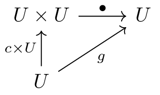
1. Firstly $U$ can encode/decode data from/to any other object in the category. This is captured in the property of it being a universal object, meaning every object of the category is a retract of $U$. 2. Secondly, $U$ has a Turing morphism $\bullet: U \times U \rightarrow U$. This can be thought of as where the computation happens. In particular, we can think of $\bullet$ as taking in two pieces of data, compiling the first piece into a program and running it on the second piece. 3. Finally, this rudimentary “computer” is universal, in the sense that it has a code (a total map $c: 1 \rightarrow U$) for every map in the category. This is stated as saying that for any $g: U \rightarrow U$ there is a code $c : 1 \rightarrow U$ s.t.

As we saw in the last article in this series, Turing categories constructed in this way are the minimal categorical setting for the central notions of computability theory enshrined in the Universality Theorem and (ameter Theorem of classical recursion theory.

Why total maps matter

So Turing categories give us a general categorical setting for computation. They let us study results like Universality and Parameter Theorems in the abstract and to disentangle classical recursion and computation theory from their historical roots over the natural numbers. This alone is quite an achievement but any computer scientist knows that there are more questions to ask about computation than can be answered just by studying recursion. The authors of this post, for example, spend most of our days wondering about not just computable functions but ones which are computable efficiently. It is probably unreasonable to expect that questions as earthly as those of efficiency and complexity are to be answered at the high level of generality of Turing categories but we can instead ask where we might look in a Turing category to find more structured forms of computation.

The total maps subcategory of a Turing category is a great candidate for a source of interesting structure. From a categorical point of view they this subcategory obeys stronger closure properties (as we’ll see later). From a computational point, total maps seem more structured because they don’t have a halting problem or undecidability in the same way that general computable maps do. So they are in a sense the most general setting for questions of complexity.

Now that we have motivation to study these total map subcategories, we want to know what they look like and how they behave. This is what brings us to the paper at hand, which provides necessary and sufficient conditions for any category to occur as the total maps of a Turing category. This investigation comes in two parts. In the first part, we look at the relationship between a total maps category and its Turing category, which is generalised in the paper into the notion of a Totalizing Extension. This will allow us to see how to import the categorical structure of the Turing category onto the total maps category, giving the necessary conditions. The second part shows these conditions to be sufficient by taking an interesting and much more computational approach. We will see in this section how to build a computational device called a stack machine inside a category with our desired conditions. This allows for a step-by-step notion of computation in the category. We can use this (under certain mild assumptions) to reconstruct the Turing application map necessary to realise our category as the total maps of a Turing category. The next two sections of this post will focus on these two parts of the story.

Totalizing extensions: constructing partial maps around your category

So we know why total maps might be an interesting object of study but how do we tell if a given category (in general without a Turing object or even a restriction structure) can be obtained as the total maps category of a Turing category? To answer this, we’re going to first need a way of talking about all the restriction categories who have our desired category as their total maps subcategory. These will be called totalizing extensions of the category. By setting this up in the right way and looking at a crucial example (which we’ll call $\hat{\mathbb{X}}$), we will see that totalizing extensions of $\mathbb{X}$ are indeed a category with $\hat{\mathbb{X}}$ as a terminal object. This then heavily constrains any totalizing extension of $\mathbb{X}$ and we will conclude this section by how these constraints can help us to detect a Turing Category in the category of totalizing extension of $\mathbb{X}$.

Motivating totalizing extensions The idea here is that for any $\mathbb{X}$ we really want to study the collection $\mathbf{TE}(\mathbb{X})$ which captures all restriction categories $\mathbb{Y}$ s.t. $\mathbf{Total}(\mathbb{Y}) \cong \mathbb{X}$. You might say at this point, “Well that seems like a fine definition for totalizing extension, why aren’t we just done?”. The problem with this definition is that it doesn’t give us a very structured set. As category theorists what are we supposed to do with $\mathbf{TE}(\mathbb{X})$ with its different restriction structures which seem to have little common categorical structure to hold them together. Instead, we want to generalise, to a purely categorical level, the properties of a functor of the form $\mathbf{Total}(\mathbb{Y}) \hookrightarrow \mathbb{Y}$. This will give us a notion of totalizing extension which doesn’t rely on arbitrary restriction categories and as we’ll see the resulting collection $\mathbf{Ext}_{\mathcal{T}}(\mathbb{X})$ will contain $\mathbf{TE}(\mathbb{X})$ and will have much more useful structural properties.

What exactly is a totalizing extension? So we want a definition for a functor $T: \mathbb{X} \rightarrow \mathbb{X}^{\prime}$ which looks like a functor $\mathbf{Total}(\mathbb{Y}) \hookrightarrow \mathbb{Y}$ but with the catch of only being able to use purely categorical notions in our definition (i.e. nowhere referring to a restriction structure). The solution given in the paper is the following:

A functor $T : \mathbb{X} \rightarrow \mathbb{X}^{\prime}$ is totalizing when it satisfies the following three conditions:

• $T$ on objects, $\text{TObj} : \text{Obj}(\mathbb{X}) \rightarrow \text{Obj}(\mathbb{X}^{\prime})$, is an isomorphism

• $T$ is faithful

• $T$ is left factor closed, meaning that when $Th = gf$ then there is a (necessarily unique) $k$ such that $Tk = f$.

Understanding the first two parts of the definition is easy. $T$ should be an isomorphism on objects because in the restriction categories setting, all identities maps are by definition total. $T$ should be faithful because the notion we’re trying to generalise is an inclusion functor. This leaves the last condition, left factor closedness. This is where we pinpoint exactly what is categorically special about total maps (separate from their definition in terms of the restriction combinator). The condition boils down to a simple slogan about composition: “if a total map $h$ can be decomposed as first doing $f$ then doing $g$ then $f$ must be itself a total map”. This definition clearly captures all the inclusion functors in what we called $\mathbf{TE}(\mathbb{X})$ but also, as we’ll see in the rest of this section, this definition gives us enough category theoretic structure to make $\mathbf{Ext}_{\mathcal{T}}(\mathbb{X})$ an interesting object to study. However, before we get on to studying this we need to answer a more basic question.

Does every category have a totalizing extension? We now find ourselves in one of the more unenviable positions of mathematics: we have a nice definition for an object we want to study ($\mathbf{Ext}_{\mathcal{T}}(\mathbb{X})$) but for all we know this object might be empty set in most cases! Here we shall put this worry to rest. To do this we take any (small) category $\mathbb{X}$ and build up a restriction category around it for which $\mathbb{X}$ is the category of total maps. A good first suggestion might recall from Cockett and Lack’s restriction categories paper that there is (or seems to be) such a construction which was called $\text{Par}(\mathbb{X})$. This category is the category of left monic cospans over $\mathbb{X}$, i.e. diagrams of the form

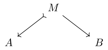
Where here we think of a partial function from $A$ to $B$ as being a function from some subobject $M$ of $A$ to $B$ and total maps are simply maps $A \rightarrow B$ in $\mathbb{X}$. Excellent! So we can just use $\mathbb{X} \hookrightarrow \text{Par}(\mathbb{X})$ as our prototypical totalizing extension?

Well, not quite. This seems ideal but there is one hitch: composition in $\text{Par}(\mathbb{X})$ relies on the existence of pullbacks in $\mathbb{X}$ so this doesn’t work for every $\mathbb{X}$. This is annoying but luckily Yoneda can come to our rescue! Indeed, we use the fact that the presheaf category $\mathbf{Set}^{\mathbb{X}^{\text{op}}}$ has all finite limits to construct a totalizing extension $\tilde{\eta}: \mathbf{Set}^{\mathbb{X}^{\text{op}}} \rightarrow \text{Par}(\mathbf{Set}^{\mathbb{X}^{\text{op}}})$ and now observe the following square that we get from the Yoneda embedding.

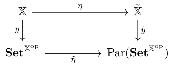
Let’s unpack that a little:

• $\mathbf{Set}^{\mathbb{X}^{\text{op}}}$ is the category whose objects are functors $F: \mathbb{X}^{\text{op}} \rightarrow \mathbf{Set}$ with natural transformations as morphisms.
• $\text{Par}(\mathbf{Set}^{\mathbb{X}^{\text{op}}})$ also has the contravariant $\mathbf{Set}$-valued functors on $\mathbb{X}$ as objects but the morphisms are left monic cospans of natural transformations
• $y$ is the Yoneda embedding of $\mathbb{X}$ into $\mathbf{Set}^{\mathbb{X}^{\text{op}}}$ as the objects $\mathbb{X}(-, A)$ for $A \in \text{Obj}(\mathbb{X})$
• $\tilde{\mathbb{X}}$ is defined as the restriction of $\text{Par}(\mathbf{Set}^{\mathbb{X}^{\text{op}}})$ to the image of $\tilde{\eta} \circ y$ on objects. i.e. it is the category with objects $\mathbb{X}(-, A)$ for $A \in \text{Obj}(\mathbb{X})$ and morphisms are left monic cospans whose apexes are general presheaves of $\mathbb{X}$

It is not hard to see that this trick does indeed work and $\eta: \mathbb{X} \rightarrow \tilde{\mathbb{X}}$ is a totalizing extension! So now we have a definite example of a totalizing extension for every category $\mathbb{X}$ and we can rest easy that $\mathbf{Ext}_{\mathcal{T}}(\mathbb{X})$ is not the empty set. Indeed, it is much more than that…

$\mathbf{Ext}_{\mathcal{T}}(\mathbb{X})$ is a category! It’s true and as we’ll see it is the structure of this category that allows Cockett, Hofstra and HrubeÅ¡ to set up the main results of this paper. To see this we first need to ask: what morphism between totalizing extensions $T: \mathbb{X} \rightarrow \mathbb{Y}$ and $T^{\prime}: \mathbb{X} \rightarrow \mathbb{Y}^{\prime}$?. The naive answer should be a diagram of the form

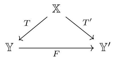
The extra condition required of $F$ is that it reflects the total maps identified by each of the extensions. The most important consequences of this definition (and confirmation in a sense that it is the “right” definition) is the following surprising fact about our innocuous example from the last paragraph:

For any $\mathbb{X}$, $\mathbf{Ext}_{\mathcal{T}}(\mathbb{X})$ is a finitely complete category with $\eta: \mathbb{X} \rightarrow \tilde{\mathbb{X}}$ as its terminal object.

This result is a pretty amazing boon to our search for a Turing category whose total maps are $\mathbb{X}$. Why is this? Well now we know that any restriction category whose total maps are like $\mathbb{X}$ will be appear as a totalizing extension $T$ in $\mathbf{Ext}_{\mathcal{T}}(\mathbb{X})$ and that in this category there will be a unique comparison map $K_T: T \rightarrow \eta$. In brief, this means that if we are lucky enough for $\mathbf{Ext}_{\mathcal{T}}(\mathbb{X})$ to contain a Turing category, then we can “project” its computational structure onto $\tilde{\mathbb{X}}$ in a unique way. This gives us a powerful rephrasing of our search for a Turing category containing $\mathbb{X}$ and one which has almost entirely abstracted away the choice of restriction structure on such a Turing category. The following result appears as Proposition 2.5 in the Cockett, Hofstra, and HrubeÅ¡ paper

$\mathbb{X}$ is the total maps of a Turing category if and only if $\tilde{\mathbb{X}}$ contains a combinatory algebra whose total computable maps include the maps of $\mathbb{X}$

This clearly still contains some restriction and computation theory but we’ll see in the next section how this result gives us full categorical necessary conditions for $\mathbb{X}$ to be the total maps of a Turing category and in the section after that we’ll see how this result is used again to show sufficiency of these conditions.

The key categorical properties of a total maps category

In this section we will identify the main conditions imposed on a category if its category of totalizing extensions contains a Turing category. The main result of the paper is that these conditions are necessary and sufficient for a category to be the total maps category of some Turing Category. As given in the paper, the conditions are as follows, a category $\mathbb{X}$ can be the total maps of a Turing category only if:

• (TM1) $\mathbb{X}$ is Cartesian
• (TM2) $\mathbb{X}$ has a universal object $U$ (i.e. for any $A$ there is a monic $\iota_A: A \hookrightarrow U$)
• (TM3) $U$ has a pair of disjoint elements $\mathbf{t}, \mathbf{f}: 1 \rightarrow U$
• (TM4) $U$ is equipped with an abstract retract structure $\mathcal{R}$
• (TM5) $\mathcal{R}$ has codes

Some of the conditions named here are quite involved so if you’re interested please check out the original paper for details as I’ll just aim to provide some intuition as to what parts of Turing categories they correspond to.

The first three conditions can all be observed just by thinking about Turing categories (forgetting the nice structure of $\mathbf{Ext}_{\mathcal{T}}(\mathbb{X})$ as a category for the moment). Indeed we know that $\mathbb{X}$ must

• be Cartesian as the restriction Cartesian structure on $\mathbb{T}$ becomes a proper restriction structure when there is no partiality.
• contain a universal object, as this is just the Turing object where the required monics exist because of the retractions $(\iota_A, \rho_A)$ in $\mathbb{T}$ and are total because $\rho_A \circ \iota_A = 1_A$
• has two “disjoint” elements of $U$ from the fact that the combinatory algebra given by $(U, \bullet)$ in $\mathbb{T}$ has codes for the two disjoint terms $\mathbf{t} = \lambda xy.x$ and $\mathbf{f} = \lambda xy.y$

The slightly more interesting (and harder to explain!) conditions (TM4 & TM5) are those relating to abstract retract structures and codes. Where do these come from? Well the easiest explanation is that there is some structure of the Turing category (for example the existence of retraction maps $\rho_A$) which doesn’t necessarily survive the restriction to total maps. In these cases, we need to use the result of the last section to observe the effects of this structure on $\mathbb{X}$. That is, we project the structure from $\mathbb{T}$ to $\tilde{\mathbb{X}}$ using the comparison functor in $\mathbf{Ext}_{\mathcal{T}}(\mathbb{X})$. With this in mind we can state (if not fully understand the details) that the abstract retract structure condition is the image of the true retract structure on $\mathbb{T}$ and the codes for this structure come from the codes $1 \rightarrow U$ which identify computable maps in $\mathbb{T}$. As both of these conditions are in a sense “filtered through” $\tilde{\mathbb{X}}$ they become quite unwieldy statements about collections of cospans of presheaves on $\mathbb{X}$. The reader is invited to check these out if they time and brain cells to spare.

Building a Turing category from the total maps conditions

Up to this point, we’ve had the goal of taking an inherently computational object (namely the total maps of a Turing category) and distilling from its computational properties, an abstract categorical understanding of its structure. In the last section we saw that the author’s of this paper really did achieve that, finding a list of categorical properties held by any category which shows up as total maps subcategory of some Turing category. In this section we would like to see that tape run in reverse. That is: we now have a category satisfying (TM1)-(TM5) and we want to rebuild some notion of computation. Stated more precisely our aim is the following:

Aim: Given a category $\mathbb{X}$ satisfying the conditions TM1-TM5, construct a PCA in $\tilde{\mathbb{X}}$ s.t. the maps of $\mathbb{X}$ are totally computable in this PCA.

In essence, we are given $\mathbb{X}$ as the remnants of some Turing category and we’re tasked with bringing the Turing category back to life. The problem is Turing categories are a very refined notion of computation so we won’t try obtain our PCA by building a Turing machine directly, instead we’ll use the parts of $\mathbb{X}$ to build different computational beast. The name of this Frankenstein’s monster is a stack machine.

Stack objects and stack machines The idea behind the “monster” that we’re about to construct is the following: if we can have an object $A$ whose data can be encoded and decoded repeatedly into itself like a stack, then we might be able to build a “machine” which performs simple “steps” which can be chained together using this stack to create a complete notion of computation. In the next short definitions we will see how this is made into a reality.

Firstly, we define a stack object in a category to be an object $A$ with an embedding retraction pair $(\texttt{put},\texttt{get}): 1 + A \times A \prec A$. We think of this as a list structure in the following way. When $\texttt{put}$ting, we are taking either the empty list $\text{nil}$ or a piece of paired data from $A \times A$ which we think of as a head followed by a tail and we encode this with a single piece of data in $A$. When $\texttt{get}$ting we are reversing this process. An important fact about these objects is that for any such object and any polynomial $P(A)$ over $+$ and $\times$ we can build an encoding decoding scheme $P(A) \prec A$. Thus stack objects allow us to encode and decode seemingly arbitrary strings of data whose signature is fixed by some polynomial $P(A)$. Crucially, the universal object $U$ guaranteed by the conditions on $\mathbb{X}$ is an example of such an object.

To make this notion useful for computation we need to build from it the notion of stack machine. A stack machine built on a stack object $A$ has a state of type $A \times A \times A$ (the parts are called the code, the data and the stack), three embedding-retraction pairs for interpreting and modifying states (one for encoding/decoding stacks as above, one for encoding/decoding instructions stored in the head of the stack and one for encoding/decoding code instructions) and a transition table which defines (as per the cases determined by the signatures for code, stack and head above) a transition $\texttt{step}: A\times A \times A \rightarrow A + A \times A \times A$ which takes the current state to a next state or an output. Choosing a good set of signatures and writing a transition table is similar to writing a compiler for a small programming language so we won’t burden this blog with a detailed example but the example (with 9 case distinctions) can be seen in the paper.

What we are going to spend time explaining is how we go from this simple transition system to a partial combinatory algebra. The first thing that might trouble us is that, in building a PCA, we’re looking for a (partially defined) application function

$\bullet: A \times A \rightarrow A$

but the only element of computation we have in a stack machine seems to be this “step” function from $A\times A \times A$ to $A + A \times A \times A$.

To compute $\mathbf{x} \bullet \mathbf{y}$ on a stack machine we need to effectively set up our machine with $\mathbf{x}$ in the code part, $\mathbf{y}$ in the value part and $\text{nil}$ in the stack and keep running “step” until we get an output (or if it doesn’t halt $\mathbf{x} \bullet \mathbf{y}$ is undefined, which is allowed). To do this in the category $\tilde{\mathbb{X}}$ we rely on the fact that such presheaf categories are traced on coproduct meaning that for any $f: X \rightarrow X + Y$ we have $f^{\dagger}: X \rightarrow Y$ which is defined as the pushout over all the partial maps $f^{i}: X \rightarrow Y$ representing the output after $i$ steps. Using this traced structure, we can define $\mathbf{x} \bullet \mathbf{y}$ as $\text{step}^{\dagger}(\mathbf{x}, \mathbf{y}, \text{nil})$.

The detail of showing that this set-up does indeed define a PCA in $\tilde{\mathbb{X}}$ and that the PCA contains $\mathbb{X}$ in its total maps relies on the details of how the transition table is programmed and on the remaining conditions on $\mathbb{X}$ but hopefully this has given a taste of how this monster is put together. Those looking to assemble their own should consult the details in the paper.

So here we are. If you take the details omitted here on faith, we have now seen that the conditions (TM1)-(TM5) are not only necessary but also sufficient for $\mathbb{X}$ to be the total maps of a Turing category. So we’ve seen the full result of this paper, a categorical characterisation of the total maps categories that we set out to understand. Now what can we do with this?

How to apply this result and where it might lead

Now that we truly understand these total map categories, we can revisit the questions we had earlier about the place of complexity in the theory of Turing categories. Indeed, a lot of the questions we might have are of the form “Does category $X$, which arises as a complexity class of maps on $\mathbb{N}$, appear as the total maps of a Turing category?”. Such questions were the focus of Cockett et al.’s paper on Timed Sets and now we have a very powerful theorem with which to answer them. In fact, for the purposes of this section, the theorem is a little too strong and so will use a helpful sufficient condition given as a corollary to the main result as Proposition 5.1:

Given a Cartesian category $\mathbb{X}$ in which:

(i). Every object has at least one element

(ii). There is a universal object $U$

(iii). There is a monic (set) map $c: \coprod_{A\in \mathbb{X}} \mathbb{X}(A, U) \rightarrow \mathbb{X} (1,U)$

(iv). There is a faithful product preserving functor $I: \mathbb{X} \rightarrow \mathbf{Set}$

Then $\mathbb{X}$ occurs as the total maps of a Turing category

This condition opens up all manner of examples of classes of maps in $\mathbf{Comp}(\mathbb{N})$ (the computable maps between powers of $\mathbb{N}$). Indeed, in such a category (i) is trivial, (iii) follows from the Gödel numbering of computable functions and (iv) is trivial as $\mathbf{Comp}(\mathbb{N})$ is a subcategory of $\mathbf{Set}$. So the main obstruction is the universality of $\mathbb{N}$ in such a category. This is resolved (and thus we can find the category as a total maps category of a Turing category) if there is a pairing map $\mathbb{N} \times \mathbb{N} \rightarrow \mathbb{N}$ in the complexity class being examined. This means that easily we have that $\textsc{linear}, \textsc{ ptime}, \textsc{ exptime}$ are all the total maps categories of some Turing categories. Similar arguments would follow as well for deterministic space complexity classes, however this seems to be only using a tiny amount of the power of the result derived. What about categories that are not derived from $\mathbf{Set}$ but still have complexity theoretic origins, for example non-deterministic complexity classes (given as subcategories of $\mathbf{Rel}$) for instance, what does this general theorem have to say about them?

To conclude, the result we’ve seen in reviewing this paper takes the pure notion of computation described by Turing categories and gives a complete classification of the total maps categories that arise in this general world. Along the way we’ve seen a mixing and merging of tricks from both category theory and computability (and even a small programming language thrown in!). However, even with this full classification, it is still difficult to get a grasp on the full extent of possible total maps categories. The examples we see from complexity theory seem to barely stretch the limits of the result proved. The authors of this post look forward to testing this result against other categories that arise as we ourselves tread the boundary between computation and category theory — and we hope you will too.