Skip to the Main Content

Note:These pages make extensive use of the latest XHTML and CSS Standards. They ought to look great in any standards-compliant modern browser. Unfortunately, they will probably look horrible in older browsers, like Netscape 4.x and IE 4.x. Moreover, many posts use MathML, which is, currently only supported in Mozilla. My best suggestion (and you will thank me when surfing an ever-increasing number of sites on the web which have been crafted to use the new standards) is to upgrade to the latest version of your browser. If that's not possible, consider moving to the Standards-compliant and open-source Mozilla browser.

December 7, 2019

Random Permutations (Part 7)

Posted by John Baez

Last time I computed the expected number of cycles of length kk in a random permutation of an nn-element set. The answer is wonderfully simple: 1/k1/k for all k=1,,nk = 1, \dots, n.

As Mark Meckes pointed out, this fact is just a shadow of a more wonderful fact. Let C kC_k be the number of cycles of length kk in a random permutation of an nn-element set, thought of as a random variable. Then as nn \to \infty, the distribution of C kC_k approaches a Poisson distribution with mean 1/k1/k.

But this is just a shadow of an even more wonderful fact!

First, if we fix some number b1b \ge 1, and look at all the random variables C 1,,C bC_1, \dots, C_b, they converge to independent Poisson distributions as nn \to \infty.

In fact we can even let bb \to \infty as nn \to \infty, so long as nn outstrips bb, in the following sense: b/n0b/n \to 0. The random variables C 1,,C bC_1, \dots , C_b will still converge to independent Poisson distributions.

These facts are made precise and proved here:

In the proof they drop another little bombshell. Suppose jkj \ne k. Then the random variables C jC_j and C kC_k become uncorrelated as soon as nn gets big enough for a permutation of an nn-element set to have both a jj-cycle and a kk-cycle. That is, their expected values obey

E(C jC k)=E(C j)E(C k) E(C_j C_k) = E(C_j) E(C_k)

whenever nj+kn \ge j + k. Of course when n<j+kn \lt j + k it’s impossible to have both a cycle of length jj and one of length kk, so in that case we have

E(C jC k)=0 E(C_j C_k) = 0

It’s exciting to me how the expected value E(C jC k)E(C_j C_k) pops suddenly from 00 to E(C j)E(C k)=1/jkE(C_j) E(C_k) = 1/jk as soon as our set gets big enough to allow both a jj-cycle and a kk-cycle. It says that in some sense the presence of a large cycle in a random permutation does not discourage the existence of other large cycles… unless it absolutely forbids it!

This is a higher-level version of a phenomenon we’ve already seen: E(C k)E(C_k) jumps from 00 to 1/k1/k as soon as nkn \ge k.

More generally, Arratia and Tavaré show that

E(C j 1C j m)=E(C j 1)E(C j m) E(C_{j_1} \, \cdots \, C_{j_m}) = E(C_{j_1}) \, \cdots \,E(C_{j_m})

whenever nj 1++j mn \ge j_1 + \cdots + j_m. But on the other hand, clearly

E(C j 1C j m)=0 E(C_{j_1} \, \cdots \, C_{j_m}) = 0

whenever n<j 1++j mn \lt j_1 + \cdots + j_m, at least if the numbers j ij_i are distinct. After all, it’s impossible for a permutation of a finite set to have cycles of different lengths that sum to more than the size of that set.

I’m trying to understand the nature of random permutations. These results help a lot. But instead of describing how they’re proved, I want to conclude with a picture that has also helped me a lot:

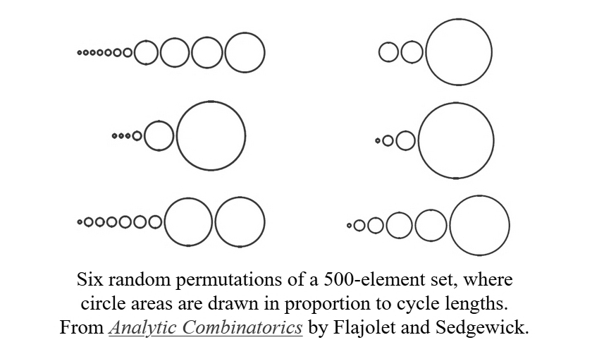
One can argue that Flajolet and Sedgewick should have used circumferences rather than areas to indicate cycle lengths: after all, the circumference is a kind of ‘cycle length’. That would have made the large cycles seem even larger compared to the puny ones.

Of course, experts on the visual display of quantitative information have a lot of opinions on these issues. But never mind! Let’s extract some morals from this chart.

We can see that a random permutation of a large set has rather few cycles on average. To be precise, the expected number of cycles in a random permutation of an nn-element set is lnn\sim \ln n.

We can also see that the lengths of the cycles range dramatically from tiny to large. To be precise, suppose 1mmn1 \le m \le m' \le n. Then since the expected number of cycles of length kk is 1/k1/k, the expected number of cycles of length between mm and mm' is close to

lnmlnm \ln m' \; - \; \ln m

Thus we can expect as many cycles of length between 11 and 1010 as between 1010 and 100100, or between 100100 and 10001000, etc.

So, I’m now imagining a random permutation of a large set as a way of chopping up a mountain into rocks with a wild range of sizes: some sand grains, some pebbles, some fist-sized rocks and some enormous boulders. Moreover, as long as two different sizes don’t add up to more than the size of our mountain, the number of rocks of those two sizes are uncorrelated.

I want to keep improving this intuition. For example, if jkj \ne k and nj+kn \ge j + k, are the random variables C jC_j and C kC_k independent, or just uncorrelated?

Posted at December 7, 2019 11:25 PM UTC

TrackBack URL for this Entry:   https://golem.ph.utexas.edu/cgi-bin/MT-3.0/dxy-tb.fcgi/3173

6 Comments & 0 Trackbacks

Re: Random Permutations (Part 7)

Maybe some of you can help me understand (and thereby prove) Equations 5 and 6 in Arratia and Tavare’s paper. They cite another paper for this equation, from a journal on population biology! But I think it should be easy and fun to figure out ourselves.

These equations concern the random variable C kC_k that I was discussing: the number of cycles of length kk in a random permutation of an nn-element set. It’s a formula for expected values of products of such random variables.

We take a list of numbers m 1,,m m_1 , \dots, m_\ell and compute the expected value of the random variable

C 1 m̲ 1C m̲ C_1^{\underline{m}_1} \cdots C_\ell^{\underline{m}_\ell}

where the underline indicates ‘falling powers’:

x m̲=x(x1)(x2)(xm+1) x^\underline{m} = x(x-1)(x-2) \cdots (x-m+1)

Equation 5 says that

E(C 1 m̲ 1C m̲ = k=1 (1k) m k E(C_1^{\underline{m}_1} \cdots C_\ell^{\underline{m}_\ell} = \prod_{k = 1}^\ell \left( \frac{1}{k} \right)^{m_k}

or in other words

E( k=1 C k m̲ k)= k=1 (1k) m k E\left( \prod_{k = 1}^\ell C_k^{\underline{m}_k} \right) = \prod_{k = 1}^\ell \left( \frac{1}{k} \right)^{m_k}

if m 1+2m 2++m nm_1 + 2 m_2 + \cdots + \ell m_\ell \le n. It also says that if this inequality is violated, the expected value is 00. So, the main thing I need to understand is this equation.

But then, in Equation 6, they reformulate this equation very suggestively as follows, given that the inequality holds:

E( k=1 C k m̲ k)=E( k=1 Z k m̲ k) E\left( \prod_{k = 1}^\ell C_k^{\underline{m}_k} \right) = E\left(\prod_{k = 1}^\ell Z_k^{\underline{m}_k}\right)

where the Z kZ_k are independent Poisson distributions with means 1/k1/k. To see why this reformulation works, I just need to see why

E(Z k n̲)=(1k) n E\left(Z_k^{\underline{n}}\right) = \left( \frac{1}{k} \right)^{n}

This must be a famous thing about Poisson distributions. I think I’ve even used it before in my own work. I bet one proof uses Dobiński’s formula for the number of partitions of an nn-element set. If we go this route, I’ll probably need to use the relation between partitions and permutations to figure out what’s really going on here.

Posted by: John Baez on December 8, 2019 7:18 AM | Permalink | Reply to this

Re: Random Permutations (Part 7)

Hi John,

a combinatorial way for looking on such relations is given by the so-called Weingarten calculus, which gives the Haar state (for example, the uniform counting measure on the permutation groups) in terms of summing over partitions of sets. In my paper Stochastic aspects of easy quantum groups with Teo Banica and Steve Curran we reproved the result for the cycles on the permutation group via such combinatorial means; however, the focus there is actually on quantum group versions of the permutation and also the orthogonal group. The nice thing is that one can treat all those objects in the same way; the difference is just the set of partitions which are involved; for the classical permutation group this is the set of all partitions, for the orthogonal group it is the subset of all pairings (matchings), and for the quantum versions one has to replace partitions by non-crossing partitions.

Posted by: Roland Speicher on December 8, 2019 11:46 AM | Permalink | Reply to this

Re: Random Permutations (Part 7)

Thanks, Roland! I’m especially interested in the case of the hyperoctahedral groups, since like the symmetric groups these are Coxeter groups. There’s a third infinite sequence of Coxeter groups, the D nD_n series. I wonder how things work for those.

Posted by: John Baez on December 12, 2019 7:47 AM | Permalink | Reply to this

Re: Random Permutations (Part 7)

Here are a bunch of facts I want to understand and somehow ‘unify’. My goal is to understand how permutations, partitions and the Poisson distribution are connected. These are some tidbits that seem to hint at a deep connection.

1) Let PP be the Poisson distribution of mean 11. Then the nnth moment of PP is the number of partitions of an nn-element set. In other words:

E[P n]= k=0 nS(n,k) E[P^n] = \sum_{k=0}^n S(n,k)

where S(n,k)S(n,k) is the number of partitions of nn into kk parts. This is sometimes called Dobiński’s formula.

More generally let P(x)P(x) be the Poisson distribution of mean xx. Then

E[P(x) n]= k=0 nS(n,k)x k E[P(x)^n] = \sum_{k=0}^n S(n,k) x^k

I don’t really understand these facts. I know how to relate Gaussian integrals to combinatorics using Feynman diagrams. Something similar should be going on here: there should be some nice way to see why moments of a Poisson distribution are governed by partitions of nn into kk parts. I know that Poisson distributions can be seen as the Fock space description of coherent states, so I have hopes.

2) Consider the falling power

x n̲=x(x1)(x2)(xn+1) x^\underline{n} = x(x-1)(x-2) \cdots (x-n+1)

which is the number of injections nxn \hookrightarrow x when xx is an integer. It obeys a formula like this:

x n= k=0 nS(n,k)x k̲ x^n = \sum_{k=0}^n S(n,k) x^{\underline k}

where S(n,k)S(n,k) is the number of partitions of nn into kk parts.

It’s enough to prove this equation for natural numbers since polynomials are equal if they agree on all natural numbers. If xx is a natural number we can prove the equation as follows.

Interpret xx as a finite set and x nx^n as the set of functions nxn \to x. Any such function has an epi-mono factorization which is unique up to isomorphism. That is, it’s given by some surjection nkn \to k, which gives a partition of kk into nn parts, followed by an injection knk \hookrightarrow n. If we count the number of options (paying careful attention to avoid overcounting) we get the right side of the above equation.

This argument goes back to Rota.

3) Putting 1) and 2) together we get

E[P n̲]=1 E[P^{\underline{n}}] = 1

Conversely, this and 2) imply 1). Wikipedia’s proof of 1) reduces it to proving E[P n̲]=1E[P^{\underline{n}}] = 1 in this way, and then quits there. This is not entirely satisfying!

4) On the other hand,

x n̲= k=0 ns(n,k)x k x^\underline{n} = \sum_{k=0}^n s(n,k) x^k

where s n,ks_{n,k} is (1) nk(-1)^{n-k} times the number of permutations of nn with exactly kk disjoint cycles. This is a kind of ‘inverse transform’, reversing the change of basis from polynomials x k̲x^{\underline k} to polynomials x nx^n given in 2). But what’s really going on here, combinatorially?

Posted by: John Baez on December 8, 2019 9:00 PM | Permalink | Reply to this

Re: Random Permutations (Part 7)

The fact that moments of the Poisson distribution are given in terms of partitions of sets comes quite naturally from the ”law of small numbers”, i.e., from the limit theorem that ((11n)δ 0+1nδ 1)) *n((1-\frac 1n)\delta_0+\frac 1n \delta_1))^{*n} converges for nn\to\infty to the Poisson distribution. If you calculate the moments in the limit of this convolutions, then they are given in terms of partitions. Doing the same for the central limit theorem, gives you the moments in the limit in terms of pairings, which is the Wick formula for Gaussian variables.

This is all kind of folklore knowledge going probably back to the beginnings of limit theorems, but since the modern machinery of Fourier transforms has taken over, it is a bit hard to find such combinatorial approaches in standard textbooks. Let me thus shamelessly refer to my own lecture notes on free probability theory, where Theorem 2.16 gives such a statement with proof. (Actually, again the main focus is there on the free analogue, but the proof for the classical statement and the free statement is in parallel, one using all partitions, the other just non-crossing partitions.)

Posted by: Roland Speicher on December 9, 2019 4:57 PM | Permalink | Reply to this

Re: Random Permutations (Part 7)

This sounds like what I need to read! For some reason I’m just seeing this comment now. I want a combinatorial approach because I’m hoping I can extract some wisdom from it.

Posted by: John Baez on December 12, 2019 7:52 AM | Permalink | Reply to this

Post a New Comment