The n-Category Café

Recall the story from last time. The Riemann sphere $\mathbb{C}\mathrm{P}^1$ consists of a copy of $\mathbb{C}$ centered at $0$ together with a point at infinity, or ‘north pole’:

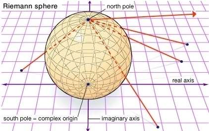
You can think of the sphere here as your eyeball, with the north pole being your optic nerve. The complex numbers $\mathbb{C}$ are like a movie screen. Light streaming in from the movie screen hits your eyeball, and each point on your eyeball gets hit… except your optic nerve.

So, $\mathbb{C}$ consists of all points of $\mathbb{C}\mathrm{P}^1$ except $\infty$. But there is also an ‘antipodal’ copy of $\mathbb{C}$ consisting of all the points in $\mathbb{C}\mathrm{P}^1$ except $0$. Imagine another plane tangent to the north pole of the sphere in the picture above, and you’ll get what I mean. Conformal inversion, the map $z \mapsto z^{-1}$, gives a bijection between these two copies of $\mathbb{C}$.

This picture lets us describe four subgroups of the group of conformal transformations of the Riemann sphere:

• rotations of the sphere $\mathbb{C}\mathrm{P}^1$ that fix the points $0$ and $\infty$
• translations of the copy of $\mathbb{C}$ containing $0$: these fix the point $\infty$
• translations of the copy of $\mathbb{C}$ containing $\infty$: these fix the point $0$
• dilations that fix the points $0$ and $\infty$.

The group of conformal transformations of the Riemann sphere is $\mathrm{PSL}(2,\mathbb{C})$, and as described last time, it’s isomorphic to the connected Lorentz group $\mathrm{SO}_0(3,1)$.

Thus, these four subgroups give four Lie subalgebras of $\mathfrak{so}(3,1) \cong \mathfrak{sl}(2,\mathbb{C})$. And the cool part is that they add up to the whole thing:

$$\mathfrak{so}(3,1) \cong \mathfrak{so}(2) \oplus \mathbb{C} \oplus \mathbb{C} \oplus \mathbb{R}$$

as vector spaces. As a quick sanity check, note that the dimensions add up correctly:

$$6 = 1 + 2 + 2 + 1$$

since the dimension of $\mathfrak{so}(3,1)$ is $4 \times 3 / 2 = 6$.

We now want to modify this story, replacing $\mathbb{C}\mathrm{P}^1$ by $\mathbb{O}\mathrm{P}^2$. This involves two changes. We need to replace $\mathbb{C}$ with $\mathbb{O}$. But the bigger change is to replace 1 by 2 — that is, replace a projective line with a projective plane.

From $\mathbb{C}\mathrm{P}^1$ to $\mathbb{O}\mathrm{P}^1$

First let me quickly indicate what happens if we just replace $\mathbb{C}$ with $\mathbb{O}$. There’s a space $\mathbb{O}\mathrm{P}^1$, which is an 8-sphere just as $\mathbb{C}\mathrm{P}^1$ is a 2-sphere. When you give this 8-sphere its round metric it has a group of conformal transformations. This group is isomorphic to $\mathrm{SO}_0(9,1)$, the identity component of the Lorentz group of 10d Minkowski spacetime. But this group is also isomorphic to $\mathrm{PSL}(2,\mathbb{O})$. Since the octonions are nonassociative, we need to work a bit to define $\mathrm{PSL}(2,\mathbb{O})$. I did it one way here:

• $\mathbb{O}\mathrm{P}^1$ and Lorentzian geometry.

but you can see another approach here:

• Tevian Dray and Corinne A. Manogue, Octonionic Cayley spinors and $\mathrm{E}_6$, Section 2: the Lorentz group.

This paper is also worth looking at for the story about $\mathbb{O}\mathrm{P}^2$.

You can think of $\mathbb{O}\mathrm{P}^1$ as a copy of $\mathbb{O}$ together with a point at infinity. But there’s also an ‘antipodal’ copy of $\mathbb{O}$ sitting in $\mathbb{O}\mathrm{P}^1$, centered at the point at infinity. These two copies of $\mathbb{O}$ are related by conformal inversion:

$$z \mapsto z^{-1}$$

All this is just like the complex case. If you’re a mathematician, you can visualize it by looking at this picture:

and imagining that both the 2-dimensional surfaces are 8-dimensional.

And just like in the complex case, we can see four subgroups of $\mathrm{PSL}(2,\mathbb{O})$, or in other words the identity component of the Lorentz group $SO(9,1)$, which acts as conformal transformations of $\mathbb{O}\mathrm{P}^1$:

• rotations of the sphere $\mathbb{O}\mathrm{P}^1$ that fix the points $0$ and $\infty$
• translations of the copy of $\mathbb{O}$ containing $0$: these fix the point $\infty$
• translations of the copy of $\mathbb{O}$ containing $\infty$: these fix the point $0$
• dilations of the copy of $\mathbb{O}$ containing $0$: these fix the points $0$ and $\infty$, and also act as dilations of the copy of $\mathbb{O}$ containing $\infty.$

These four subgroups give four Lie subalgebras of $\mathfrak{so}(3,1)$ that add up to the whole thing:

$$\mathfrak{so}(9,1) \cong \mathfrak{so}(8) \oplus \mathbb{O} \oplus \mathbb{O} \oplus \mathbb{R}$$

As a quick check, note that the dimensions add up correctly:

$$45 = 28 + 8 + 8 + 1$$

since the dimension of $\mathfrak{so}(9,1)$ is $10 \times 9 / 2 = 45$ while that of $\mathfrak{so}(8)$ is $8 \times 7 / 2 = 28$.

From $\mathbb{C}\mathrm{P}^1$ to $\mathbb{C}\mathrm{P}^2$

Now let’s do something harder: replacing the projective line $\mathbb{C}\mathrm{P}^1$ by the projective plane $\mathbb{C}\mathrm{P}^2$. The big difference is that while a projective line is just an ordinary line together with a point at infinity, a projective plane is an ordinary plane together with a line at infinity (which is a projective line). We used inversion to switch between two copies of $\mathbb{C}$ sitting $\mathbb{C}\mathrm{P}^1$: one centered at $0$ and one centered at $\infty$. To copy this trick for $\mathbb{C}\mathrm{P}^2$, we need to also use the duality between points and lines — a special feature of projective plane geometry.

Projective planes are a wonderful distillation of some old thoughts in axiomatic geometry. You’ve got a set of ‘points’, a set of ‘lines’, and a relation saying when a point ‘lies on a line’. You’ve got two axioms:

• any two distinct points lie on a unique line.
• any two distinct lines have a unique point lying on both of them.

These axioms are self-dual: for any projective plane $P$ there’s a dual projective plane $P^\ast$ such that points of $P$ are lines of $P^\ast$ and vice versa, and the ‘lies on’ relation is reversed! So we’re in a situation that really takes advantage of Hilbert’s remark on the arbitrariness of names in formal mathematics:

One must be able to say at all times — instead of ‘points’, ‘straight lines’, and ‘planes’ — ‘tables’, ‘chairs’, and ‘beer mugs’.

In projective plane geometry, instead of points and lines, one can say ‘lines’ and ‘points’, and all the theorems are still true!

Here’s how you get a projective plane from a field $\mathbb{F}$. You take a 3-dimensional vector space $U$ over $\mathbb{F}$. You define ‘points’ to be 1-dimensional subspaces of $U$, and ‘lines’ to be the 2-dimensional subspaces of $U$, and you say a point $p$ ‘lies on’ a line $\ell$ iff $p \subseteq \ell$. The resulting projective plane is called the projectivization of $U$, or $P U$.

What if we replace the vector space $U$ with its dual $U^\ast$? I’ll let you check: a point in $P U^\ast$ corresponds to a line in $P U$, and vice versa, and the ‘lies on’ relation is reversed. So we have a natural isomorphism

$$P (U^\ast) \cong (P U)^\ast$$

where the dual at right is the dual for projective planes. Of course every finite-dimensional vector space is isomorphic to its dual, so we also have $U^\ast \cong U$ and thus $(P U)^\ast \cong P U$. But these are not natural isomorphisms.

Now let’s take our field $\mathbb{F}$ to be $\mathbb{C}$, and take $U = \mathbb{C}^3$.

We get a projective plane $\mathbb{C}\mathrm{P}^2$, but also a dual projective plane $(\mathbb{C}\mathrm{P}^2)^\ast$: points in one are lines in the other. $\mathbb{C}\mathrm{P}^2$ consists of $\mathbb{C}^2$ together with a line at infinity, say $\ell_\infty$. Right in the middle of $\mathbb{C}^2$ is the origin, $0$. Since it’s a point let’s call it $p_0$. So:

$$p_0 \in \mathbb{C}^2 \cong \mathbb{C}\mathrm{P}^2 - \{\ell_\infty\}$$

But the point $p_0$ in $\mathbb{C}\mathrm{P}^2$ corresponds to a line in $(\mathbb{C}\mathrm{P}^2)^\ast$! If we remove this line we’re left with a copy of $(\mathbb{C}^2)^\ast$ — do you see why? And $\ell_\infty$ is sitting inside this $(\mathbb{C}^2)^\ast$. So:

$$\ell_\infty \in (\mathbb{C}^2)^\ast \cong (\mathbb{C}\mathrm{P}^2)^\ast - \{p_0\}$$

In short, the situation is wonderfully symmetrical.

Now, the group $\mathrm{SL}(3,\mathbb{C})$ acts as linear transformations of both $\mathbb{C}^3$ and its dual. These are non-isomorphic representations of $\mathrm{SL}(3,\mathbb{C})$, which is why I’m being so careful to distinguish them. We get actions of $\mathrm{PSL}(3,\mathbb{C})$ on the projective plane $\mathbb{C}\mathrm{P}^2$ and on the dual projective plane $(\mathbb{C}\mathrm{P}^2)^\ast$. And these let us describe four subgroups of $\mathrm{PSL}(3,\mathbb{C})$:

• transformations in $\mathrm{SL}(2,\mathbb{C})$: these fix $p_0$ and $\ell_\infty$, and act linearly on $\mathbb{C}^2$ and $(\mathbb{C}^2)^\ast$
• translations of the copy of $\mathbb{C}^2$ containing $p_0$: these fix $\ell_\infty$
• translations of the copy of $(\mathbb{C}^2)^\ast$ containing $\ell_\infty$: these fix $p_0$
• ‘complex dilations’, i.e. transformations of $\mathbb{C}^2$ of the form $v \mapsto c v$ for $c \in \mathbb{C}^\ast$: these also act as complex dilations of $(\mathbb{C}^2)^*$, and they fix both $p_0$ and $\ell_\infty.$

By analogy with what we’ve seen so far, we could hope for an isomorphism of vector spaces

$$\mathfrak{sl}(3,\mathbb{C}) \cong \mathfrak{sl}(2,\mathbb{C}) \oplus \mathbb{C}^2 \oplus (\mathbb{C}^2)^\ast \oplus \mathbb{C}$$

And in fact it’s true! I won’t prove it here, but it’s not hard. Each of the four pieces at right at right is a Lie subalgebra of $\mathfrak{sl}(3,\mathbb{C})$, but they don’t all commute with each other so this is not an isomorphism of Lie algebras.

As a check we can see if the dimensions add up correctly… and they do!

$$8 = 3 + 2 + 2 + 1$$

We can also think of this in terms of groups and group representations. $\mathrm{SL}(2,\mathbb{C})$ is the double cover of the connected Lorentz group $\mathrm{SO}_0(3,1)$, and $\mathbb{C}^2$ and $(\mathbb{C}^2)^\ast$ are its right-handed and left-handed spinor representations — called Weyl spinors. So, in some sense we can chop $\mathrm{PSL}(3,\mathbb{C})$ into four parts:

• the double cover of the Lorentz group in 4 dimensions
• translations in left-handed spinor directions
• translations in right-handed spinor directions
• complex dilations.

But this is easier to make rigorous at the Lie algebra level, where $\mathfrak{sl}(3,\mathbb{C})$ is the direct sum of four subspaces that happen to be Lie subalgebras:

• the Lorentz Lie algebra $\mathfrak{so}(3,1)$
• right-handed Weyl spinors: $\mathbb{C}^2$
• left-handed Weyl spinors: $(\mathbb{C}^2)^\ast$
• complex scalars: $\mathbb{C}$

From $\mathbb{C}\mathrm{P}^2$ to $\mathbb{O}\mathrm{P}^2$

The octonions are not a field, but the story I just told generalizes from $\mathbb{C}\mathrm{P}^2$ to $\mathbb{O}\mathrm{P}^2$.

The projective plane $\mathbb{O}\mathrm{P}^2$ has a dual, $(\mathbb{O}\mathrm{P}^2)^\ast$. Points in $\mathbb{O}\mathrm{P}^2$ are lines in the dual, and vice versa. $\mathbb{O}\mathrm{P}^2$ consists of $\mathbb{O}^2$ together with a line at infinity, say $\ell_\infty$. Right in the middle of $\mathbb{O}^2$ is the origin, which we’ll call $p_0$. So:

$$p_0 \in \mathbb{O}^2 \cong \mathbb{O}\mathrm{P}^2 - \{\ell_\infty\}$$

But the point $p_0$ in $\mathbb{O}\mathrm{P}^2$ corresponds to a line in $(\mathbb{O}\mathrm{P}^2)^\ast$. If we remove this line from $(\mathbb{O}\mathrm{P}^2)^\ast$ we’re left with a copy of $(\mathbb{O}^2)^\ast$, and we get

$$\ell_\infty \in (\mathbb{O}^2)^\ast \cong (\mathbb{O}\mathrm{P}^2)^\ast - \{p_0\}$$

The group of symmetries (technically ‘collineations’) of the projective plane $\mathbb{O}\mathrm{P}^2$ is our friend $\mathrm{E}_6$. This also acts on the dual projective plane. Using this fact we get four subgroups of $\mathrm{E}_6$, almost like in the complex case:

• transformations in $\mathrm{SL}(2,\mathbb{O})$: these fix $p_0$ and $\ell_\infty$, and act linearly on $\mathbb{O}^2$ and $(\mathbb{O}^2)^\ast$
• translations of the copy of $\mathbb{O}^2$ containing $p_0$: these fix $\ell_\infty$
• translations of the copy of $(\mathbb{O}^2)^\ast$ containing $\ell_infty$: these fix $p_0$
• dilations, i.e. transformations of $\mathbb{O}^2$ of the form $v \mapsto c v$ for $c \in \mathbb{R}^\ast$: these also act as dilations of $(\mathbb{O}^2)^*$, and they fix both $p_0$ and $\ell_\infty$.

Following the pattern, we could hope for that the Lie algebras of these subgroups add up to give the whole Lie algebra of $\mathrm{E}_6$. And it’s true!

$$\mathfrak{e}_6 \cong \mathfrak{sl}(2,\mathbb{O}) \oplus \mathbb{O}^2 \oplus (\mathbb{O}^2)^\ast \oplus \mathbb{R}$$

Again, each of of the four pieces at right is a Lie subalgebra of $\mathfrak{e}_6$, but they don’t all commute with each other so this is not an isomorphism of Lie algebras.

As a sanity check we can see if the dimensions add up correctly. In fact I already did this back in Part 7. So, its Lie algebra has dimension $10 \times 9 / 2 = 45$, and the sum goes like this:

$$78 = 45 + 16 + 16 + 1$$

And we saw another way to think about this stuff. $\mathrm{SL}(2,\mathbb{O})$ is the double cover of the connected Lorentz group $\mathrm{SO}_0(9,1)$, better known as $\mathrm{Spin}(9,1)$. The spaces $\mathbb{O}^2$ and $(\mathbb{O}^2)^\ast$ are the right-handed and left-handed spinor representations of $\mathrm{Spin}(9,1)$, called Majorana–Weyl spinors. So, what we’re doing is breaking the Lie algebra $\mathfrak{e}_6$ into four parts, that happen to be Lie subalgebras:

• the Lorentz Lie algebra $\mathfrak{so}(9,1)$
• right-handed Majorana–Weyl spinors: $\mathbb{O}^2$
• right-handed Majorana–Weyl spinors: $(\mathbb{O}^2)^\ast$
• scalars: $\mathbb{R}$

Okay, I hope the picture is reasonably clear by now — though there is still work required to check everything, which I haven’t done here. If I were being more systematic I’d generalize this story to the projective spaces $\mathbb{K}\mathrm{P}^n$ for all normed division algebras $\mathbb{K} = \mathbb{R}, \mathbb{C}, \mathbb{H}, \mathbb{O}$ — for all $n$ when $\mathbb{K}$ is associative, but only $n = 1,2,3$ when $\mathbb{K} = \mathbb{O}$. In higher dimensions there’s a duality between points and $(n-1)$-dimensional projective subspaces. But the story is most interesting to me when it involves the coincidences

$$\begin{array}{ccl} \mathrm{PSL}(2,\mathbb{R}) & \cong & \mathrm{SO}_0(2,1) \\ \mathrm{PSL}(2,\mathbb{C}) & \cong & \mathrm{SO}_0(3,1) \\ \mathrm{PSL}(2,\mathbb{H}) & \cong & \mathrm{SO}_0(5,1) \\ \mathrm{PSL}(2,\mathbb{O}) & \cong & \mathrm{SO}_0(9,1) \end{array}$$

And right now I’m just interested in the complex and octonionic cases, which are linked by these inclusions:

$$\begin{array}{ccccccc} \mathrm{PSL}(2,\mathbb{C}) & \subset & \mathrm{PSL}(2,\mathbb{O}) \\ \cap & & \cap \\ \mathrm{PSL}(3,\mathbb{C})& \subset & \mathrm{PSL}(3,\mathbb{O}) \\ \end{array}$$

with $\mathrm{PSL}(3,\mathbb{O})$ being a nickname for $\mathrm{E}_6$.

---

• Part 1. How to define octonion multiplication using complex scalars and vectors, much as quaternion multiplication can be defined using real scalars and vectors. This description requires singling out a specific unit imaginary octonion, and it shows that octonion multiplication is invariant under $\mathrm{SU}(3)$.
• Part 2. A more polished way to think about octonion multiplication in terms of complex scalars and vectors, and a similar-looking way to describe it using the cross product in 7 dimensions.
• Part 3. How a lepton and a quark fit together into an octonion — at least if we only consider them as representations of $\mathrm{SU}(3)$, the gauge group of the strong force. Proof that the symmetries of the octonions fixing an imaginary octonion form precisely the group $\mathrm{SU}(3)$.
• Part 4. Introducing the exceptional Jordan algebra $\mathfrak{h}_3(\mathbb{O})$: the $3 \times 3$ self-adjoint octonionic matrices. A result of Dubois-Violette and Todorov: the symmetries of the exceptional Jordan algebra preserving their splitting into complex scalar and vector parts and preserving a copy of the $2 \times 2$ adjoint octonionic matrices form precisely the Standard Model gauge group.
• Part 5. How to think of $2 \times 2$ self-adjoint octonionic matrices as vectors in 10d Minkowski spacetime, and pairs of octonions as left- or right-handed spinors.
• Part 6. The linear transformations of the exceptional Jordan algebra that preserve the determinant form the exceptional Lie group $\mathrm{E}_6$. How to compute this determinant in terms of 10-dimensional spacetime geometry: that is, scalars, vectors and left-handed spinors in 10d Minkowski spacetime.
• Part 7. How to describe the Lie group $\mathrm{E}_6$ using 10-dimensional spacetime geometry. This group is built from the double cover of the Lorentz group, left-handed and right-handed spinors, and scalars in 10d Minkowski spacetime.
• Part 8. A geometrical way to see how $\mathrm{E}_6$ is connected to 10d spacetime, based on the octonionic projective plane.
• Part 9. Duality in projective plane geometry, and how it lets us break the Lie group $\mathrm{E}_6$ into the Lorentz group, left-handed and right-handed spinors, and scalars in 10d Minkowski spacetime.
• Part 10. Jordan algebras, their symmetry groups, their invariant structures — and how they connect quantum mechanics, special relativity and projective geometry.
• Part 11. Particle physics on the spacetime given by the exceptional Jordan algebra: a summary of work with Greg Egan and John Huerta.