Skip to the Main Content

Note:These pages make extensive use of the latest XHTML and CSS Standards. They ought to look great in any standards-compliant modern browser. Unfortunately, they will probably look horrible in older browsers, like Netscape 4.x and IE 4.x. Moreover, many posts use MathML, which is, currently only supported in Mozilla. My best suggestion (and you will thank me when surfing an ever-increasing number of sites on the web which have been crafted to use the new standards) is to upgrade to the latest version of your browser. If that's not possible, consider moving to the Standards-compliant and open-source Mozilla browser.

December 16, 2020

Octonions and the Standard Model (Part 10)

Posted by John Baez

The Dynkin diagram of E 6\mathrm{E}_6 has 2-fold symmetry:

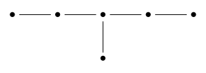
So, this Lie group has a nontrivial outer automorphism of order 2. This corresponds to duality in octonionic projective plane geometry! There’s an octonionic projective plane 𝕆P 2\mathbb{O}\mathrm{P}^2 on which E 6\mathrm{E}_6 acts. But there’s also a dual octonionic projective plane (𝕆P 2) *(\mathbb{O}\mathrm{P}^2)^*. Points in the dual plane are lines in the original one, and vice versa. And these two projective planes are not isomorphic as spaces on which the group E 6\mathrm{E}_6 acts. Instead, there’s a bijection

α:𝕆P 2(𝕆P 2) * \alpha : \mathbb{O}\mathrm{P}^2 \to (\mathbb{O}\mathrm{P}^2)^*

such that acting by gE 6g \in \mathrm{E}_6 and then applying α\alpha is the same as applying α\alpha and then acting by gE 6g' \in \mathrm{E}_6, where gg' is what you get when you apply the outer automorphism to gg.

Similarly, the group E 6\mathrm{E}_6 acts on the exceptional Jordan algebra and its dual, but these are not isomorphic as representations of E 6\mathrm{E}_6. Instead they’re only isomorphic up to an outer automorphism.

Today I want to tell you about invariant structures on the exceptional Jordan algebra and its dual. But a lot of this stuff applies more generally.

The exceptional Jordan algebra 𝔥 3(𝕆)\mathfrak{h}_3(\mathbb{O}) consists of self-adjoint 3×33 \times 3 matrices of octonions. But many facts about it also work if we replace the octonions by any normed division algebra. So let 𝕂\mathbb{K} be any normed division algebra, meaning ,,\mathbb{R}, \mathbb{C}, \mathbb{H} or 𝕆\mathbb{O}. And let 𝔥 3(𝕂)\mathfrak{h}_3(\mathbb{K}) be the space of self-adjoint 3×33 \times 3 matrices with entries in 𝕂\mathbb{K}. Explicitly:

𝔥 3(𝕂)={(α z y * z * β x y x * γ):x,y,z𝕂,α,β,γ} \mathfrak{h}_3(\mathbb{K}) = \left\{ \left( \begin{array}{ccc} \alpha & z & y^\ast \\ z^\ast & \beta & x \\ y & x^\ast & \gamma \end{array} \right) : \; x,y,z \in \mathbb{K}, \alpha, \beta, \gamma \in \mathbb{R} \right\}

This vector space has a cubic form, the determinant

det(α z y * z * β x y x * γ)=αβγ(α|x| 2+β|y| 2+γ|z| 2)+2Re(xyz) \mathrm{det} \left( \begin{array}{ccc} \alpha & z & y^\ast \\ z^\ast & \beta & x \\ y & x^\ast & \gamma \end{array} \right) = \alpha \beta \gamma - (\alpha |x|^2 + \beta |y|^2 + \gamma |z|^2) + 2 Re(x y z)

which, we’ve seen, is well-defined even when 𝕂\mathbb{K} is not associative. It’s also a formally real Jordan algebra with Jordan product

ab=12(ab+ba)a,b𝔥 3(𝕂) a \circ b = \frac{1}{2} (a b + b a) \qquad a,b \in \mathfrak{h}_3(\mathbb{K})

where aba b stands for the usual product of 3×33 \times 3 matrices.

While it’s not obvious, there’s a formula for the determinant in terms of the product. So we have two symmetry groups:

  • the Lorentz group, consisting of linear transformations of 𝔥 3(𝕂)\mathfrak{h}_3(\mathbb{K}) that preserve the determinant,
  • the automorphism group, consisting of linear transformations of 𝔥 3(𝕂)\mathfrak{h}_3(\mathbb{K}) that preserve the Jordan product, and

and the former contains the latter.

Both groups are important, because we can use formally real Jordan algebras for two purposes: as algebras of observables, and as spacetimes! These Jordan algebras were invented to describe observables in quantum mechanics:

From this viewpoint, the important symmetry group is the automorphism group.

But these Jordan algebras are also vector spaces with very symmetrical cones, generalizing the light-cone in Minkowski spacetime:

  • J. Faraut and A. Korányi, Analysis on Symmetric Cones, Oxford University Press, Oxford, 1994.

From this viewpoint, the important symmetry group is the Lorentz group, since it generalizes the Lorentz group we know and love from special relativity.

All this is very clear if we look at the Jordan algebra 𝔥 2(𝕂)\mathfrak{h}_2(\mathbb{K}), which consists of 2×22 \times 2 self-adjoint matrices with entries in 𝕂\mathbb{K}. I’ve already discussed in Part 8. Instead of showing you the Lorentz group and automorphism group of 𝔥 2(𝕂)\mathfrak{h}_2(\mathbb{K}), let me just show you their Lie algebras, to eliminate some distracting fluff:

𝕂 LorentzLiealgebraof𝔥 2(𝕂) derivationLiealgebraof𝔥 2(𝕂) 𝔰𝔩(2,)𝔰𝔬(2,1) 𝔰𝔲(2,)𝔰𝔬(2) 𝔰𝔩(2,)𝔰𝔬(3,1) 𝔰𝔲(2,)𝔰𝔬(3) 𝔰𝔩(2,)𝔰𝔬(5,1) 𝔰𝔲(2,)𝔰𝔬(5) 𝕆 𝔰𝔩(2,𝕆)𝔰𝔬(9,1) 𝔰𝔲(2,𝕆)𝔰𝔬(9) \begin{array}{lcc} \mathbb{K} \quad & Lorentz \; Lie \; algebra \; of \; \mathfrak{h}_2(\mathbb{K}) & derivation \; Lie \; algebra \; of \; \mathfrak{h}_2(\mathbb{K}) \\ \\ \mathbb{R} & \mathfrak{sl}(2,\mathbb{R}) \cong \mathfrak{so}(2,1) & \mathfrak{su}(2,\mathbb{R}) \cong \mathfrak{so}(2) \\ \mathbb{C} & \mathfrak{sl}(2,\mathbb{C}) \cong \mathfrak{so}(3,1) & \mathfrak{su}(2,\mathbb{C}) \cong \mathfrak{so}(3) \\ \mathbb{H} & \mathfrak{sl}(2,\mathbb{H}) \cong \mathfrak{so}(5,1) & \mathfrak{su}(2,\mathbb{H}) \cong \mathfrak{so}(5) \\ \mathbb{O} & \mathfrak{sl}(2,\mathbb{O}) \cong \mathfrak{so}(9,1) & \mathfrak{su}(2, \mathbb{O}) \cong \mathfrak{so}(9) \\ \end{array}

Here 𝕙 2(𝕂)\mathbb{h}_2(\mathbb{K}) is the algebra of observables for a real, complex, quaternionic or octonionic qubit. So its automorphism group consists roughly of 2×22 \times 2 unitary matrices with entries in 𝕂\mathbb{K}, mod phase… just as you’d expect for the symmetrices of qubits of these sort. But 𝕙 2(𝕂)\mathbb{h}_2(\mathbb{K}) is also Minkowski spacetime of dimension 2+1,3+1,5+12+1, 3+1, 5+1 or 9+19+1: the determinant of these 2×22 \times 2 matrices provides the Minkowski metric. So its Lorentz group is just the usual Lorentz group for Minkowski spacetime of that dimension. The automorphism group is a subgroup of that, consisting of Lorentz transformations that fix the time axis: the orthogonal group in dimension 2, 3, 4 or 9.

Why did I say “roughly”? When dealing with Lie groups we always have worry about how many connected components we want, and also which quotient group of the universal cover. Also everything has to be interpreted carefully in the octonionic case. But the main point is: we’re seeing the two faces of these Jordan algebras: they’re algebras of observables and also spacetimes.

And there’s a third face: these Jordan algebras 𝕙 2(𝕂)\mathbb{h}_2(\mathbb{K}) give projective lines! Elements of a Jordan algebra with pp=pp \circ p = p are called projections. For 𝕙 2(𝕂)\mathbb{h}_2(\mathbb{K}) they come in three kinds: those with trace 0, those with trace 1 and those with trace 2. There’s only one with trace 0 and it’s boring: just 0, the additive identity in our Jordan algebra. There’s only one with trace 2 and it’s boring: just 1, the multiplicative identity in our Jordan algebra. The interesting ones have trace 1, and these correspond to points of the projective line 𝕂P 1\mathbb{K}\mathrm{P}^1.

All this is just a warmup for what I’m really interested in, 𝕙 3(𝕂)\mathbb{h}_3(\mathbb{K}) and its connection to the projective plane 𝕂P 2\mathbb{K}\mathrm{P}^2. Here’s what we get in that case:

𝕂 LorentzLiealgebraof𝔥 3(𝕂) derivationLiealgebraof𝔥 3(𝕂) 𝔰𝔩(3,) 𝔰𝔲(3,) 𝔰𝔩(3,) 𝔰𝔲(3,) 𝔰𝔩(3,) 𝔰𝔲(3,) 𝕆 𝔢 6 𝔣 4 \begin{array}{lcc} \mathbb{K} \quad & Lorentz \; Lie \; algebra \; of \; \mathfrak{h}_3(\mathbb{K}) & derivation \; Lie \; algebra \; of \; \mathfrak{h}_3(\mathbb{K}) \\ \\ \mathbb{R} & \mathfrak{sl}(3,\mathbb{R}) & \mathfrak{su}(3,\mathbb{R}) \\ \mathbb{C} & \mathfrak{sl}(3,\mathbb{C}) & \mathfrak{su}(3,\mathbb{C}) \\ \mathbb{H} & \mathfrak{sl}(3,\mathbb{H}) & \mathfrak{su}(3,\mathbb{H}) \\ \mathbb{O} & \mathfrak{e}_6 & \mathfrak{f}_4 \end{array}

There’s a nice simple pattern, except for the octonions!

And except for the octonions, there’s no need to limit ourselves to 3×33 \times 3 matrices: the self-adjoint m×mm \times m matrices 𝔥 m(𝕂)\mathfrak{h}_m(\mathbb{K}) have a perfectly fine determinant and Jordan product for all mm, so we can work at this level of generality. The quaternions are a bit annoying because they’re not a field, but one can work around this. So, let’s talk about 𝔥 m(𝕂)\mathfrak{h}_m(\mathbb{K}), and its Lorentz and automorphism groups, for 𝕂=,\mathbb{K} = \mathbb{R}, \mathbb{C} and \mathbb{H}.

The Jordan algebras 𝔥 m(𝕂)\mathfrak{h}_m(\mathbb{K}) are algebras of observables for real, complex, and quaternionic quantum systems. But they are also exotic ‘spacetimes’ where the lightcone is defined by the equation

det(a)=0 \det (a) = 0

When m=2m = 2 this is a quadratic equation and we get a Minkowski spacetime. When m=3m = 3 we get a cubic equation, and that’s the case I’m most interested in today. And the story continues for higher mm.

These Jordan algebras also give projective geometries! I’ll just say how how it goes for m=3m = 3, where they give projective planes. The projections in 𝔥 3(𝕂)\mathfrak{h}_3(\mathbb{K}) come in four kinds. There’s one with trace 0, namely 0. There’s a bunch with trace 1, and these are points of the projective plane 𝕂P 2\mathbb{K}\mathrm{P}^2. There’s a bunch with trace 2, and these are lines in the projective plane 𝕂P 2\mathbb{K}\mathrm{P}^2. And there’s one with trace 3, namely 1. I hope you can guess how this generalizes for higher mm.

Here’s how the Lorentz group works for 𝔥 m(𝕂)\mathfrak{h}_m(\mathbb{K}). First, define the general linear group GL(m,𝕂)\mathrm{GL}(m,\mathbb{K}) to be the group of invertible m×mm \times m matrices with entries in 𝕂\mathbb{K}. Then define the special linear group SL(m,𝕂)\mathrm{SL}(m,\mathbb{K}) to be the commutator subgroup of GL(m,𝕂)\mathrm{GL}(m,\mathbb{K}) When 𝕂\mathbb{K} is the real or complex numbers, SL(m,𝕂)\mathrm{SL}(m,\mathbb{K}) is the same as the group of m×mm \times m matrices with determinant 1, and it’s obvious that SL(m,𝕂)\mathrm{SL}(m,\mathbb{K}) acts on 𝔥 m(𝕂)\mathfrak{h}_m(\mathbb{K}) as follows:

g:agag * g: a \to g a g^\ast

It’s also obvious that this action preserves the determinant. All this is also true in the quaternionic case if one uses the correct approach to quaternionic determinants — a rabbit hole into which I’d rather not hop. Unfortunately, SL(m,𝕂)\mathrm{SL}(m,\mathbb{K}) is not exactly the group of determinant-preserving transformations of 𝔰𝔩(m,𝕂)\mathfrak{sl}(m,\mathbb{K}) — there are some discrete subgroup subtleties which I’ll mention later — but I’m pretty sure it has the right Lie algebra. We call this Lie algebra 𝔰𝔩(m,𝕂)\mathfrak{sl}(m,\mathbb{K}) the Lorentz Lie algebra of 𝔥 m(𝕂)\mathfrak{h}_m(\mathbb{K}).

Here’s how the automorphism group works. First, define the special unitary group SU(m,𝕂)\mathrm{SU}(m,\mathbb{K}) to be the subgroup of SL(m,𝕂)\mathrm{SL}(m,\mathbb{K}) consisting of matrices that are ‘unitary’ in the sense that gg *=g *g=1g g^\ast = g^\ast g = 1. Such matrices act as automorphisms of 𝔥 m(𝕂)\mathfrak{h}_m(\mathbb{K}) as follows:

agag *=gag 1 a \mapsto g a g^\ast = g a g^{-1}

Now, SU(m,𝕂)\mathrm{SU}(m,\mathbb{K}) is not exactly the automorphisms of 𝔥 m(𝕂)\mathfrak{h}_m(\mathbb{K}) — again there are some annoying subtleties — but it has the right Lie algebra. We call this Lie algebra 𝔰𝔲(m,𝕂)\mathfrak{su}(m,\mathbb{K}) the derivation Lie algebra of 𝔥 m(𝕂)\mathfrak{h}_m(\mathbb{K}).

So, we have these for all mm:

𝕂 LorentzLiealgebraof𝔥 m(𝕂) derivationLiealgebraof𝔥 m(𝕂) 𝔰𝔩(m,) 𝔰𝔲(m,) 𝔰𝔩(m,) 𝔰𝔲(m,) 𝔰𝔩(m,) 𝔰𝔲(m,) \begin{array}{lcc} \mathbb{K} \quad & Lorentz \; Lie \; algebra \; of \; \mathfrak{h}_m(\mathbb{K}) & derivation \; Lie \; algebra \; of \; \mathfrak{h}_m(\mathbb{K}) \\ \\ \mathbb{R} & \mathfrak{sl}(m,\mathbb{R}) & \mathfrak{su}(m,\mathbb{R}) \\ \mathbb{C} & \mathfrak{sl}(m,\mathbb{C}) & \mathfrak{su}(m,\mathbb{C}) \\ \mathbb{H} & \mathfrak{sl}(m,\mathbb{H}) & \mathfrak{su}(m,\mathbb{H}) \\ \end{array}

Invariant structures

Now let’s focus on 𝔥 3(𝕂)\mathfrak{h}_3(\mathbb{K}) and see what structures it has that are invariant under the Lorentz group. I’m really interested in the octonionic case, where 𝔥 3(𝕂)\mathfrak{h}_3(\mathbb{K}) is the exceptional Jordan algebra and this group is E 6\mathrm{E}_6, but here’s how all four cases work, I think:

𝕂 Lorentzgroupof𝔥 3(𝕂) automorphismgroupof𝔥 3(𝕂) PGL(3,) PO(3) PGL(3,)×/2 PU(3)×/2 PGL(3,) PSp(3) 𝕆 E 6 F 4 \begin{array}{lc} \mathbb{K} \quad & Lorentz \; group \; of \; \mathfrak{h}_3(\mathbb{K}) & automorphism \; group \; of \mathfrak{h}_3(\mathbb{K}) \\ \\ \mathbb{R} & \mathrm{PGL}(3,\mathbb{R}) & PO(3) \\ \mathbb{C} & \mathrm{PGL}(3,\mathbb{C}) \times \mathbb{Z}/2 & PU(3) \times \mathbb{Z}/2 \\ \mathbb{H} & \mathrm{PGL}(3,\mathbb{H}) & PSp(3) \\ \mathbb{O} & \mathrm{E}_6 & \mathrm{F}_4 \\ \end{array}

The extra factor of /2\mathbb{Z}/2 in the complex case comes from complex conjugation: we can take the complex conjugate of each entry of a self-adjoint matrix, and this operation preserves the Jordan product ab=ab+baa \circ b = a b + b a. This fails for the quaternions and octonions, because they’re noncommutative.

The next paragraph explains the rest of this chart, and I recommend skipping it unless you love collecting Lie group facts.

The group PO\mathrm{PO} is the projective orthogonal group, the orthogonal group O(n)\mathrm{O}(n) modulo its center, and for n2n \ge 2 the center of O(n)\mathrm{O}(n) is ±1\pm 1, consisting of real multiples of the identity matrix. The smelly-sounding group PU\mathrm{PU} is the projective unitary group, the unitary group U(n)\mathrm{U}(n) modulo its center, and for n1n \ge 1 the center of U(n)\mathrm{U}(n) is U(1)\mathrm{U}(1), consisting of complex multiples of the identity matrix. By PSp\mathrm{PSp}, I mean the compact symplectic group modulo its center. Concretely, the compact symplectic group Sp(n)\mathrm{Sp}(n) is the group of n×nn \times n matrices gg with quaternion entries obeying gg *=g *g=1g g^\ast = g^\ast g = 1, and PSp(n)\mathrm{PSp}(n) is Sp(n)\mathrm{Sp}(n) modulo its center, which for n1n \ge 1 is ±1\pm 1, consisting of real multiples of the identity matrix. Subtleties involving quotients by discrete subgroups are often a bit annoying, so I hasten to reassure you that the real forms of F 4\mathrm{F}_4 and E 6\mathrm{E}_6 we’re working with in these articles, namely the compact real form of F 4\mathrm{F}_4 and the noncompact form E 6(26)\mathrm{E}_{6(-26)}, have both trivial center and trivial fundamental group—so no such subtleties arise for these.

The determinant on 𝔥 3(𝕂)\mathfrak{h}_3(\mathbb{K})

The first invariant structure on 𝔥 3(𝕂)\mathfrak{h}_3(\mathbb{K}) is the determinant:

det(α z y * z * β x y x * γ)=αβγ(α|x| 2+β|y| 2+γ|z| 2)+2Re(xyz) \mathrm{det} \left( \begin{array}{ccc} \alpha & z & y^\ast \\ z^\ast & \beta & x \\ y & x^\ast & \gamma \end{array} \right) = \alpha \beta \gamma - (\alpha |x|^2 + \beta |y|^2 + \gamma |z|^2) + 2 Re(x y z)

This is a cubic form on 𝔥 3(𝕂)\mathfrak{h}_3(\mathbb{K}).

In Part 5 we saw how to write an element of 𝔥 3(𝕂)\mathfrak{h}_3(\mathbb{K}) in terms of a scalar, a vector and a left-handed spinor in (n+2)(n+2)-dimensional Minkowski spacetime, where nn is the dimension of our division algebra 𝕂\mathbb{K}: 1, 2, 4 or 8. Here scalars are elements of \mathbb{R}, vectors are elements of

V=𝔥 2(𝕂) V = \mathfrak{h}_2(\mathbb{K})

left-handed spinors are elements of

S =𝕂 2 S_- = \mathbb{K}^2

equipped with a particular representation of Spin(n+1,1)\mathrm{Spin}(n+1,1) described in Part 5, and right-handed spinors are elements of

S +=𝕂 2 S_+ = \mathbb{K}^2

made into the representation of Spin(n+1,1)\mathrm{Spin}(n+1,1) dual to the left-handed spinors. So, I’m claiming we have a specific isomorphism

𝔥 3(𝕂)VS \mathfrak{h}_3(\mathbb{K}) \cong \mathbb{R} \oplus V \oplus S_-

To get this isomorphism, the trick is to write our element

a=(α z y * z * β x y x * γ)𝔥 3(𝕂) a = \left( \begin{array}{ccc} \alpha & z & y^\ast \\ z^\ast & \beta & x \\ y & x^\ast & \gamma \end{array} \right) \in \mathfrak{h}_3(\mathbb{K})

as

a=(α ψ ψ v) a = \left( \begin{array}{cc} \alpha & \psi^\dagger \\ \psi & v \end{array} \right)

where α\alpha \in \mathbb{R} is a scalar,

v=(β x x * γ)V v = \left( \begin{array}{cc} \beta & x \\ x^\ast & \gamma \end{array} \right) \in V

is a vector, and

ψ=(z * y)S \psi = \left( \begin{array}{cc} z^\ast \\ y \end{array} \right) \in S_-

is a left-handed spinor. In Theorem 8 we saw that

det(a)=αg(v,v)+g(v,[ψ,ψ]) \mathrm{det}(a) = - \alpha g(v,v) + g(v, [\psi, \psi])

where gg is the Minkowski metric on vectors, and the bracket is an operation that eats two left-handed spinors and spits out a vector.

The trilinear form on 𝔥 3(𝕂)\mathfrak{h}_3(\mathbb{K})

We can turn any cubic form into a symmetric trilinear form! There’s a unique symmetric trilinear form

t:𝔥 3(𝕂)×𝔥 3(𝕂)×𝔥 3(𝕂) t \colon \mathfrak{h}_3(\mathbb{K}) \times \mathfrak{h}_3(\mathbb{K}) \times \mathfrak{h}_3(\mathbb{K}) \to \mathbb{R}

with

det(a)=t(a,a,a) \det(a) = t(a,a,a)

and this is invariant under the Lorentz group of 𝔥 3(𝕂)\mathfrak{h}_3(\mathbb{K}). Explicitly, if we have

a i=(α i z i y i * z i * β i x i y i x i * γ i) a_i = \left( \begin{array}{ccc} \alpha_i & z_i & y^\ast_i \\ z_i^\ast & \beta_i & x_i \\ y_i & x^\ast_i & \gamma_i \end{array} \right)

then

6t(a 1,a 2,a 3) = all6permutationsof{1,2,3}α iβ jγ k+2Re(x iy jz k) 2 i{1,2,3},with{j,k}={1,2,3}i(α iRe(x j *x k)+β iRe(y j *y k)+γ iRe(z j *z k)) \begin{array}{ccl} 6 t(a_1,a_2,a_3) &=& \displaystyle{ \sum_{all \; 6 \; permutations \; of \; \{1,2,3\}} \alpha_i \beta_j \gamma_k + 2 Re(x_i y_j z_k) - } \\ \\ & & \displaystyle{ 2 \sum_{i \in \{1,2,3\}, with \; \{j,k\} = \{1,2,3\}-i} \left( \alpha_i Re(x_j^\ast x_k) + \beta_i Re(y_j^\ast y_k) + \gamma_i Re(z_j^\ast z_k) \right) } \end{array}

Alternatively, if we write a ia_i in terms of scalars, left-handed spinors and vectors:

a i=(α i ψ i ψ i v i) a_i = \left( \begin{array}{cc} \alpha_i & \psi^\dagger_i \\ \psi_i & v_i \end{array} \right)

then we have

t(a 1,a 2,a 3) = 13 i{1,2,3},with{j,k}={1,2,3}iRe(ψ j v˜ iψ k)α ig(v j,v k) = 13 i{1,2,3},with{j,k}={1,2,3}ig(v i,[ψ j,ψ k])r ig(v j,v k) \begin{array}{rcl} t(a_1,a_2,a_3) & = & \displaystyle{ \frac{1}{3} \sum_{i \in \{1,2,3\}, with \; \{j,k\} = \{1,2,3\}-i } Re(\psi_j^\dagger \tilde{v}_i \psi_k) - \alpha_i g(v_j, v_k) } \\ \\ \\ & = & \displaystyle{ \frac{1}{3} \sum_{i \in \{1,2,3\}, with \; \{j,k\} = \{1,2,3\}-i } g(v_i, [\psi_j, \psi_k]) - r_i g(v_j, v_k) } \end{array}

These last two formulas, and any formula to come that looks a bit scary, were derived by Greg Egan using Mathematica, back in November 2015 when we were working on this stuff with John Huerta. He only did the calculations in the octonionic case, but since the other normed division algebras are subalgebras of 𝕆\mathbb{O} those cases follow!

The dual 𝔥 3(𝕂) *\mathfrak{h}_3(\mathbb{K})^\ast

The dual 𝔥 3(𝕂) *\mathfrak{h}_3(\mathbb{K})^\ast, is inequivalent to 𝔥 3(𝕂)\mathfrak{h}_3(\mathbb{K}) as a representation of the Lorentz group. So, we must carefully distinguish between them! Nonetheless, every Lorentz-invariant structure carried by one is also carried by the other, since there’s an automorphism of Lorentz group that interchanges these two representations.

We shall think of 𝔥 3(𝕂) *\mathfrak{h}_3(\mathbb{K})^\ast as consisting of 3×33 \times 3 self-adjoint matrices with entries in 𝕂\mathbb{K}, where the pairing

,:𝔥 3(𝕂) *×𝔥 3(𝕂) \langle -,- \rangle : \mathfrak{h}_3(\mathbb{K})^\ast \times \mathfrak{h}_3(\mathbb{K}) \to \mathbb{R}

is given by

h,h=12Retr(hh) \langle h', h \rangle = \frac{1}{2} Re\;tr(h' h)

This makes 𝔥 3(𝕂) *\mathfrak{h}_3(\mathbb{K})^\ast look suspiciously similar to 𝔥 3(𝕂)\mathfrak{h}_3(\mathbb{K}). Isn’t there a paradox here? No: the trace is invariant under the automorphism group of 𝔥 3(𝕂)\mathfrak{h}_3(\mathbb{K}), but not under the Lorentz group. So, while we can use the trace to identify 𝔥 3(𝕂)\mathfrak{h}_3(\mathbb{K}) with its dual, this identification is not invariant under the Lorentz group.

As a representation of Spin(n+1,1)\mathrm{Spin}(n+1,1) there is an isomorphism

𝔥 3(𝕂) *VS + \mathfrak{h}_3(\mathbb{K})^\ast \cong \mathbb{R} \oplus V \oplus S_+

under which (β,w,ϕ)VS +(\beta,w,\phi) \in \mathbb{R} \oplus V \oplus S_+ corresponds to

(β ϕ ϕ w˜)𝔥 3(𝕂) * \left( \begin{array}{cc} \beta & \phi^\dagger \\ \phi & \tilde{w} \end{array} \right) \in \mathfrak{h}_3(\mathbb{K})^\ast

where the tilde stands for ‘trace reversal’ of matrices w𝔥 2(𝕂)w \in \mathfrak{h}_2(\mathbb{K}), given by w˜=wtr(v)1\tilde{w} = w - \mathrm{tr}(v) \, 1, as in Part 6.

In these terms, the pairing

,:𝔥 3(𝕂) *×𝔥 3(𝕂) \langle -,- \rangle : \mathfrak{h}_3(\mathbb{K})^\ast \times \mathfrak{h}_3(\mathbb{K}) \to \mathbb{R}

is given as follows:

(β,w,ϕ),(α,v,ψ) = 12Retr((β ϕ ϕ w˜)(α ψ ψ v)) = 12αβ+g(v,w)+ϕ,ψ\begin{array}{rcl} \langle (\beta, w, \phi) , (\alpha, v, \psi) \rangle & = & \frac{1}{2} Re\;tr\big( \left( \begin{array}{cc} \beta & \phi^\dagger \\ \phi & \tilde{w} \end{array} \right) \left( \begin{array}{cc} \alpha & \psi^\dagger \\ \psi & v\end{array} \right) \big)\\ & = & \frac{1}{2} \alpha \beta + g(v,w) + \langle \phi, \psi \rangle \end{array}

where the angle bracket is the invariant pairing between right- and left-handed spinors, as explained in Part 6.

The cross product on 𝔥 3(𝕂)\mathfrak{h}_3(\mathbb{K})

Dualizing the trilinear form

t:𝔥 3(𝕂)×𝔥 3(𝕂)×𝔥 3(𝕂) t : \mathfrak{h}_3(\mathbb{K}) \times \mathfrak{h}_3(\mathbb{K}) \times \mathfrak{h}_3(\mathbb{K}) \to \mathbb{R}

we get a bilinear map called the cross product:

×:𝔥 3(𝕂)×𝔥 3(𝕂)𝔥 3(𝕂) * \times : \mathfrak{h}_3(\mathbb{K}) \times \mathfrak{h}_3(\mathbb{K}) \to \mathfrak{h}_3(\mathbb{K})^\ast

Beware: despite the connotations of the phrase ‘cross product’, this is a symmetric bilinear map.

We can describe the cross product explicitly, using our isomorphisms

𝔥 3(𝕂)VS \mathfrak{h}_3(\mathbb{K}) \cong \mathbb{R} \oplus V \oplus S_-

𝔥 3(𝕂) *VS + \mathfrak{h}_3(\mathbb{K})^\ast \cong \mathbb{R} \oplus V \oplus S_+

In these terms the cross product is:

(α,v,ψ)×(α,v,ψ)=13(2g(v,v),αvαv+[ψ,ψ],v˜ψ+v˜ψ) (\alpha, v , \psi) \times (\alpha', v', \psi') = \frac{1}{3} \big( -2g(v, v'), -\alpha v' - \alpha' v + [\psi , \psi'], \tilde{v} \psi' + \tilde{v'} \psi \big)

The cubic form on 𝔥 3(𝕂) *\mathfrak{h}_3(\mathbb{K})^\ast

Since 𝔥 3(𝕂) *\mathfrak{h}_3(\mathbb{K})^\ast is a kind of evil twin of 𝔥 3(𝕂)\mathfrak{h}_3(\mathbb{K}), it has its own version of everything that 𝔥 3(𝕂)\mathfrak{h}_3(\mathbb{K}) has.

For starters, it has its own version of the determinant. Namely, there is a cubic form on 𝔥 3(𝕂) *\mathfrak{h}_3(\mathbb{K})^\ast given by

det(α,ψ +,v)=αdet(v)+g(v,[ψ +,ψ +]) det'(\alpha, \psi_+, v) = \alpha det(v) + g(v, [\psi_+, \psi_+])

where now the bracket eats a pair of right-handed spinors and spits out a vector, as explained in Part 6.

The trilinear form on 𝔥 3(𝕂) *\mathfrak{h}_3(\mathbb{K})^\ast

𝔥 3(𝕂) *\mathfrak{h}_3(\mathbb{K})^\ast also has its own trilinear form. There is a unique symmetric trilinear form

t:𝔥 3(𝕂) *×𝔥 3(𝕂) *×𝔥 3(𝕂) * t' : \mathfrak{h}_3(\mathbb{K})^\ast \times \mathfrak{h}_3(\mathbb{K})^\ast \times \mathfrak{h}_3(\mathbb{K})^\ast \to \mathbb{R}

with

det(a)=t(a,a,a) det'(a) = t'(a,a,a)

and this has an explicit form that looks very similar to tt on 𝔥 3(𝕂)\mathfrak{h}_3(\mathbb{K}):

t(a 1,a 2,a 3) = 13 i{1,2,3},with{j,k}={1,2,3}iRe(s j v is k)α ig(v˜ j,v˜ k) = 13 i{1,2,3},with{j,k}={1,2,3}ig(v i,[s j,s k])α ig(v j,v k) \begin{array}{rcl} t'(a_1,a_2,a_3) & = & \displaystyle{ \frac{1}{3} \sum_{i \in \{1,2,3\}, with \; \{j,k\} = \{1,2,3\}-i } Re(s_j^\dagger v_i s_k) - \alpha_i g(\tilde{v}_j, \tilde{v}_k) } \\ \\ \\ & = & \displaystyle{ \frac{1}{3} \sum_{i \in \{1,2,3\}, with \; \{j,k\} = \{1,2,3\}-i } g(v_i, [s_j, s_k]) - \alpha_i g(v_j, v_k) } \end{array}

The second formula here appears identical to that for tt. However, the bracket operation on right-handed spinors differs from that on left-handed spinors, so it is not the same!

The cross product on 𝔥 3(𝕂) *\mathfrak{h}_3(\mathbb{K})^\ast

Dualizing the trilinear form

t:𝔥 3(𝕂) *×𝔥 3(𝕂) *×𝔥 3(𝕂) * t' : \mathfrak{h}_3(\mathbb{K})^\ast \times \mathfrak{h}_3(\mathbb{K})^\ast \times \mathfrak{h}_3(\mathbb{K})^\ast \to \mathbb{R}

we get a symmetric bilinear map, another cross product:

×:𝔥 3(𝕂) *×𝔥 3(𝕂) *𝔥 3(𝕂) \times\!' : \mathfrak{h}_3(\mathbb{K})^\ast \times \mathfrak{h}_3(\mathbb{K})^\ast \to \mathfrak{h}_3(\mathbb{K})

This has an explicit form similar to the original cross product above:

(β,w,ϕ)×(β,w,ϕ)=13(2g(w,w),βwβw+[ϕ,ϕ],wϕ+wϕ) (\beta, w, \phi) \times\!' (\beta', w', \phi') = \frac{1}{3} \big( -2g(w, w'), -\beta w' - \beta' w + [\phi , \phi'], w \phi' + w' \phi \big)

The projective plane and its dual

Last time I showed you how every projective plane has a dual, with points of the dual being lines in the original, and vice versa. I hope it’s believable that just as we can describe the projective plane 𝕂P 2\mathbb{K}\mathrm{P}^2 using 𝔥 3(𝕂)\mathfrak{h}_3(\mathbb{K}), we can describe the dual of this projective plane using the dual 𝔥 3(𝕂) *\mathfrak{h}_3(\mathbb{K})^\ast. I won’t go into the details, but I want to mention one cool thing, which I learned from this marvelous paper:

We can describe points of 𝕂P 2\mathbb{K}\mathrm{P}^2 using elements of 𝔥 3(𝕂)\mathfrak{h}_3(\mathbb{K}). I said they were projections with trace 1, but this description is only invariant under the automorphism group of 𝔥 3(𝕂)\mathfrak{h}_3(\mathbb{K}), not its Lorentz group, since it involves the Jordan product. There’s a Lorentz-invariant description too! Points of 𝕂P 2\mathbb{K}\mathrm{P}^2 correspond to equivalence classes of nonzero elements p𝔥 3(𝕂)p \in \mathfrak{h}_3(\mathbb{K}) with p×p=0p \times p = 0, where two are equivalent if one is a real multiple of the other.

Similarly, we can describe lines of 𝕂P 2\mathbb{K}\mathrm{P}^2 — that is, points of the dual plane — using certain elements of 𝔥 3(𝕂) *\mathfrak{h}_3(\mathbb{K})^\ast. They correspond to equivalence classes of nonzero elements p𝔥 3(𝕂) *p \in \mathfrak{h}_3(\mathbb{K})^\ast with p×p=0p \times' p = 0, where two are equivalent if one is a real multiple of the other.

The cross product

×:𝔥 3(𝕂)×𝔥 3(𝕂)𝔥 3(𝕂) * \times : \mathfrak{h}_3(\mathbb{K}) \times \mathfrak{h}_3(\mathbb{K}) \to \mathfrak{h}_3(\mathbb{K})^\ast

then does something really nice: for two distinct points, it gives the line through these points! And the other cross product

×:𝔥 3(𝕂) *×𝔥 3(𝕂) *𝔥 3(𝕂) \times\!' : \mathfrak{h}_3(\mathbb{K})^\ast \times \mathfrak{h}_3(\mathbb{K})^\ast \to \mathfrak{h}_3(\mathbb{K})

works dually: for two distinct lines, it gives the point lying on both lines! So, the invariant algebraic structures I’ve been discussing are secretly invariant geometrical structures.

I explain this more carefully here:

  • John Baez, The octonions. Section 3.4: 𝕆P 2\mathbb{O}\mathrm{P}^2 and the exceptional Jordan algebra.

I only talk about the octonionic case, but it works more or less the same for all four normed division algebras!

I’ve tried to sketch out how Jordan algebras serve to connect three subjects: generalizations of quantum mechanics, generalizations of special relativity, and projective geometry. I’m afraid you’ll have to look at the references to get the whole story. For more on the connection between quantum mechanics and projective geometry, try this:

I’m not quite done yet! I want to end with a few handy facts.

The action of the Lorentz group on 𝔥 3(𝕂)\mathfrak{h}_3(\mathbb{K})

In Part 7 we saw how the group E 6\mathrm{E}_6 contained four subgroups whose Lie algebra span the whole Lie algebra 𝔢 6\mathfrak{e}_6, and we described how each of these subgroups act on 𝔥 3(𝕆)\mathfrak{h}_3(\mathbb{O}). This is the octonionic case of something that works for all four normed division algebras! But there’s a slight twist in some case. It’s time to explain this now.

What I’m calling the Lorentz group of 𝔥 3(𝕂)\mathfrak{h}_3(\mathbb{K}) — that is, its group of determinant-preserving linear transformations — has the following four subgroups:

1) First, Spin(n+1,1)\mathrm{Spin}(n+1,1) can be seen as a subgroup, where nn is the dimension of 𝕂\mathbb{K}. For this we use the isomorphism

𝔥 3(𝕂)VS \mathfrak{h}_3(\mathbb{K}) \cong \mathbb{R} \oplus V \oplus S_-

described earlier and let Spin(n+1,1)\mathrm{Spin}(n+1,1) act on each of the three summands separately: they’re all representations of this group, as described in Part 5. We’ve seen the determinant is built using operations on ,V\mathbb{R}, V and S S_- that are invariant under Spin(n+1,1)\mathrm{Spin}(n+1,1).

2) Second, the vector space of right-handed spinors S +=𝕂 2S_+ = \mathbb{K}^2, regarded as an abelian Lie group, can be seen as a Lie subgroup of the Lorentz group. For this, let ϕS +\phi \in S_+ act on

(α ψ ψ v)𝔥 3(𝕂) \left( \begin{array}{cc} \alpha & \psi^\dagger \\ \psi & v \end{array} \right) \in \mathfrak{h}_3(\mathbb{K})

as follows:

v v ψ ψ+γ(vϕ) α α+g(v,[ϕ,ϕ])+2ϕ,ψ \begin{array}{ccl} v & \mapsto & v \\ \psi &\mapsto& \psi + \gamma(v \otimes \phi) \\ \alpha & \mapsto & \alpha + g(v, [\phi, \phi]) + 2 \langle \phi, \psi \rangle \end{array}

The bracket here describes a way to turn two right-handed spinors into a vector. The angle brackets denote the dual pairing between S +S_+ and S S_-, which produces a real number. And γ\gamma is a way for any vector to act on a right-handed spinor to give a left-handed spinor. We checked in Part 7 that the above action preserves the determinant in the octonionic case, and I think the same claculations work for the other normed division algebras.

3) Similarly, the space of left-handed spinors S =𝕂 2S_- = \mathbb{K}^2 can be seen as an abelian Lie subgroup of E 6\mathrm{E}_6. For this, let ηS \eta \in S_- act on

(α ψ ψ v)𝔥 3(𝕂) \left( \begin{array}{cc} \alpha & \psi^\dagger \\ \psi & v \end{array} \right) \in \mathfrak{h}_3(\mathbb{K})

as follows:

v v+12α[η,η]+[ψ,η] ψ ψ+αη α α \begin{array}{ccl} v &\mapsto& v + \frac{1}{2} \alpha [\eta, \eta] + [\psi, \eta] \\ \psi & \mapsto& \psi + \alpha \eta \\ \alpha &\mapsto& \alpha \end{array}

4) Similarly, *\mathbb{R}^\ast, the multiplicative group of nonzero real numbers, can be seen as an abelian Lie subgroup of the Lorentz group. For this, let any nonzero real number tt act on

(α ψ ψ v)𝔥 3(𝕂) \left( \begin{array}{cc} \alpha & \psi^\dagger \\ \psi & v \end{array} \right) \in \mathfrak{h}_3(\mathbb{K})

as follows:

v t 2v ψ tψ α t 4α \begin{array}{ccl} v &\mapsto& t^{-2} v \\ \psi &\mapsto& t \psi \\ \alpha &\mapsto& t^4 \alpha \end{array}

These rescalings clearly preserve the determinant, which equals αdet(v)+g(v,[ψ,ψ])\alpha \det(v) + g(v, [\psi, \psi]).

Another cool fact: we can implement actions 2)–4) by transformations on the matrix:

h=(α ψ ψ v)h = \left( \begin{array}{cc} \alpha & \psi^\dagger \\ \psi & v \end{array} \right)

that all take this form:

h12((gh)g +g(hg )) h \mapsto \frac{1}{2}((g h)g^\dagger + g (h g^\dagger))

For the action of a right-handed spinor ϕS +\phi \in S_+, we set:

g=(1 ϕ 0 1) g = \left( \begin{array}{cc} 1 & \phi \\ 0 & 1 \end{array} \right)

where the 1 in the bottom-right corner of the matrix is a 2×22 \times 2 identity matrix. For the action of a left-handed spinor ηS \eta \in S_-, we set:

g=(1 0 η 1) g = \left( \begin{array}{cc} 1 & 0 \\ \eta & 1 \end{array} \right)

And for the action of a scalar t{0}t \in \mathbb{R} - \{0\}, we set:

g=(t 2 0 0 0 t 1 0 0 0 t 1) g = \left( \begin{array}{ccc} t^2 & 0 & 0\\ 0 & t^{-1} & 0\\ 0 & 0 & t^{-1} \end{array} \right)

Now for the twist: in Theorem 9, we saw that the subgroups 1)–4) have Lie algebras that span the whole derivation Lie algebra of 𝔥 3(𝕂)\mathfrak{h}_3(\mathbb{K})in the case 𝕂=𝕆\mathbb{K} = \mathbb{O}! This also works when 𝕂=\mathbb{K} = \mathbb{R}, but when 𝕂\mathbb{K} is \mathbb{C} or \mathbb{H} we don’t get the whole thing. To get the whole thing, we should let the nonzero scalar tt above take values in \mathbb{C} or \mathbb{H}!

Though it’s not a proof, we can see evidence for this by simple dimension counting, as follows:

For 𝕂=\mathbb{K} = \mathbb{R}:

dim(𝔰𝔬(2,1))+dim(S +)+dim(S )+dim() = dim(𝔰𝔩(2,)+dim( 2)+dim( 2)+dim() = 3+2+2+1 = 8 = dim(𝔰𝔩(3,)) \begin{array}{ccl} \dim(\mathfrak{so}(2,1)) + \dim(S_+) + \dim(S_-) + \dim(\mathbb{R}) &=& \dim(\mathfrak{sl}(2,\mathbb{R}) + \dim(\mathbb{R}^2) + \dim(\mathbb{R}^2) + \dim(\mathbb{R}) \\ &=& 3 + 2 + 2 + 1 \\ &=& 8 \\ &=& \dim(\mathfrak{sl}(3,\mathbb{R})) \end{array}

For 𝕂=\mathbb{K} = \mathbb{C},

dim(𝔰𝔬(3,1))+dim(S +)+dim(S )+dim() = dim(𝔰𝔩(2,)+dim( 2)+dim( 2)+dim() = 6+4+4+2 = 16 = dim(𝔰𝔩(3,)) \begin{array}{ccl} \dim(\mathfrak{so}(3,1)) + \dim(S_+) + \dim(S_-) + \dim(\mathbb{C}) &=& \dim(\mathfrak{sl}(2,\mathbb{C}) + \dim(\mathbb{C}^2) + \dim(\mathbb{C}^2) + \dim(\mathbb{C}) \\ &=& 6 + 4 + 4 + 2 \\ &=& 16 \\ &=& \dim(\mathfrak{sl}(3,\mathbb{C})) \end{array}

For 𝕂=\mathbb{K} = \mathbb{H},

dim(𝔰𝔬(5,1))+dim(S +)+dim(S )+dim() = dim(𝔰𝔩(2,)+dim( 2)+dim( 2)+dim() = 15+8+8+4 = 35 = dim(𝔰𝔩(3,)) \begin{array}{ccl} \dim(\mathfrak{so}(5,1)) + \dim(S_+) + \dim(S_-) + \dim(\mathbb{H}) &=& \dim(\mathfrak{sl}(2,\mathbb{H}) + \dim(\mathbb{H}^2) + \dim(\mathbb{H}^2) + \dim(\mathbb{H}) \\ &=& 15 + 8 + 8 + 4 \\ &=& 35 \\ &=& \dim(\mathfrak{sl}(3,\mathbb{H})) \end{array}

For 𝕂=𝕆\mathbb{K} = \mathbb{O},

dim(𝔰𝔬(9,1))+dim(S +)+dim(S )+dim() = dim(𝔰𝔩(2,𝕆)+dim(𝕆 2)+dim(𝕆 2)+dim() = 45+16+16+1 = 78 = dim(𝔰𝔩(3,𝕆)) \begin{array}{ccl} \dim(\mathfrak{so}(9,1)) + \dim(S_+) + \dim(S_-) + \dim(\mathbb{R}) &=& \dim(\mathfrak{sl}(2,\mathbb{O}) + \dim(\mathbb{O}^2) + \dim(\mathbb{O}^2) + \dim(\mathbb{R}) \\ &=& 45 + 16 + 16 + 1 \\ &=& 78 \\ &=& \dim(\mathfrak{sl}(3,\mathbb{O})) \end{array}

where 𝔰𝔩(3,𝕆)\mathfrak{sl}(3,\mathbb{O}) is just our nickname for 𝔢 6\mathfrak{e}_6, and 𝔰𝔩(2,𝕆)\mathfrak{sl}(2,\mathbb{O}) is just our nickname for 𝔰𝔬(9,1)\mathfrak{so}(9,1).

The action of E 6\mathrm{E}_6 on 𝔥 3(𝕂) *\mathfrak{h}_3(\mathbb{K})^\ast

The action of E 6\mathrm{E}_6 on 𝔥 3(𝕂) *\mathfrak{h}_3(\mathbb{K})^\ast is very much like its action on 𝔥 3(𝕂)\mathfrak{h}_3(\mathbb{K}), but with the roles of S +S_+ and S S_- reversed.

Explicitly, we act on the matrix

h=(β ϕ ϕ w˜)h' = \left( \begin{array}{cc} \beta & \phi^\dagger \\ \phi & \tilde{w} \end{array} \right)

with the transformation:

h12((gh)g +g(hg )) h' \mapsto \frac{1}{2}((g' h')g'^\dagger + g' (h' g'^\dagger))

where:

g=(g 1) g' = (g^{-1})^\dagger

Acting this way on hh' while acting with gg on h𝔥 3(𝕆)h \in \mathfrak{h}_3(\mathbb{O}) as above preserves the pairing:

h,h=12Retr(hh)\langle h',h \rangle = \frac{1}{2} Re\;tr(h'h)


  • Part 1. How to define octonion multiplication using complex scalars and vectors, much as quaternion multiplication can be defined using real scalars and vectors. This description requires singling out a specific unit imaginary octonion, and it shows that octonion multiplication is invariant under SU(3)\mathrm{SU}(3).
  • Part 2. A more polished way to think about octonion multiplication in terms of complex scalars and vectors, and a similar-looking way to describe it using the cross product in 7 dimensions.
  • Part 3. How a lepton and a quark fit together into an octonion — at least if we only consider them as representations of SU(3)\mathrm{SU}(3), the gauge group of the strong force. Proof that the symmetries of the octonions fixing an imaginary octonion form precisely the group SU(3)\mathrm{SU}(3).
  • Part 4. Introducing the exceptional Jordan algebra 𝔥 3(𝕆)\mathfrak{h}_3(\mathbb{O}): the 3×33 \times 3 self-adjoint octonionic matrices. A result of Dubois-Violette and Todorov: the symmetries of the exceptional Jordan algebra preserving their splitting into complex scalar and vector parts and preserving a copy of the 2×22 \times 2 adjoint octonionic matrices form precisely the Standard Model gauge group.
  • Part 5. How to think of 2×22 \times 2 self-adjoint octonionic matrices as vectors in 10d Minkowski spacetime, and pairs of octonions as left- or right-handed spinors.
  • Part 6. The linear transformations of the exceptional Jordan algebra that preserve the determinant form the exceptional Lie group E 6\mathrm{E}_6. How to compute this determinant in terms of 10-dimensional spacetime geometry: that is, scalars, vectors and left-handed spinors in 10d Minkowski spacetime.
  • Part 7. How to describe the Lie group E 6\mathrm{E}_6 using 10-dimensional spacetime geometry. This group is built from the double cover of the Lorentz group, left-handed and right-handed spinors, and scalars in 10d Minkowski spacetime.
  • Part 8. A geometrical way to see how E 6\mathrm{E}_6 is connected to 10d spacetime, based on the octonionic projective plane.
  • Part 9. Duality in projective plane geometry, and how it lets us break the Lie group E 6\mathrm{E}_6 into the Lorentz group, left-handed and right-handed spinors, and scalars in 10d Minkowski spacetime.
  • Part 10. Jordan algebras, their symmetry groups, their invariant structures — and how they connect quantum mechanics, special relativity and projective geometry.
  • Part 11. Particle physics on the spacetime given by the exceptional Jordan algebra: a summary of work with Greg Egan and John Huerta.
Posted at December 16, 2020 10:16 PM UTC

TrackBack URL for this Entry:   https://golem.ph.utexas.edu/cgi-bin/MT-3.0/dxy-tb.fcgi/3265

9 Comments & 0 Trackbacks

Re: Octonions and the Standard Model (Part 10)

Glitch alert:

To get this isomorphism, the trick is write it our element

Posted by: Blake Stacey on December 17, 2020 4:07 AM | Permalink | Reply to this

Re: Octonions and the Standard Model (Part 10)

Thanks! By the way, I just updated the last section, so if you made your comment while I was doing that, you might enjoy another look.

Posted by: John Baez on December 17, 2020 6:12 AM | Permalink | Reply to this

Re: Octonions and the Standard Model (Part 10)

also Minkowski spacetime of dimension 2+1, 3+1, 4+1 or 9+1

is the third one meant to be 5+1? Else it’s not consistent with the table before it.

Posted by: David Roberts on December 17, 2020 11:52 AM | Permalink | Reply to this

Re: Octonions and the Standard Model (Part 10)

Sorry, I’ll fix that. These numbers are supposed to be 2 more than my favorite numbers: 1, 2, 4 and 8, the dimensions of ,,\mathbb{R}, \mathbb{C}, \mathbb{H} and 𝕆\mathbb{O}.

In case anyone is just tuning in:

A self-adjoint 2×22 \times 2 matrix with entries in ,,\mathbb{R}, \mathbb{C}, \mathbb{H} or 𝕆\mathbb{O} has 2 real diagonal entries and one independent off diagonal entry that can be anything, so the space of these matrices has dimension 1+2, 2+2, 4+2 or 8+2, respectively. In applications to superstring theory the 2 is the dimension of the string worldsheet and the other dimensions are the orthogonal directions in which the superstring vibrates. But one direction of the string worldsheet is timelike and all the other directions are spacelike, so physicists say the superstring is moving in a spacetime with dimension 2+1, 3+1, 5+1, or 9+1.

Needless to say, the octonionic (9+1)-dimensional case is the one that has superstring theorists really excited.

Posted by: John Baez on December 17, 2020 5:08 PM | Permalink | Reply to this

Re: Octonions and the Standard Model (Part 10)

You taught us lots about Dynkin diagrams and geometry back in the past, e.g., TWF187 and earlier weeks. I’m not sure you got onto the exceptional groups, but in week 187, you’re telling us that

the Dynkin diagram D4 is all about triality and the octonions

Does the material there help us think about E6, and understand what it has to do with the octonions?

Posted by: David Corfield on December 17, 2020 1:23 PM | Permalink | Reply to this

Re: Octonions and the Standard Model (Part 10)

Great question!

Yes, triality is hard at work behind the scenes here. The joy of the exceptional Jordan algebra is that on the one hand it’s a way of describing the octonionic projective plane — the highest-dimensional octonionic projective space allowed before nonassociativity shuts down the fun — and on the other hand it’s all about triality. This is one of nature’s miracles.

An element of the exceptional Jordan algebra looks like this:

a=(α z y * z * β x y x * γ) a = \left( \begin{array}{ccc} \alpha & z & y^\ast \\ z^\ast & \beta & x \\ y & x^\ast & \gamma \end{array} \right)

where α,β,γ\alpha, \beta, \gamma are real and x,y,zx,y,z are octonions.

So we’ve got three 8-dimensional things here. But triality is all about the group D 4=Spin(8)\mathrm{D}_4 = Spin(8) and its three 8-dimensional irreducible representations: vectors, right-handed spinors and left-handed spinors. And it turns out that if you identify x,y,x,y, and zz with those three kinds of things in an arbitrary way, all the Jordan algebra operations are invariant under Spin(8)Spin(8).

So Spin(8)Spin(8) is a very visible, tractable subgroup of the automorphism group of the exceptional Jordan algebra F 4\mathrm{F}_4, which in turn is a subgroup of its determinant-preserving transformations, E 6\mathrm{E}_6.

Another nice subgroup of F 4\mathrm{F}_4 is S 3S_3, which permutes x,y,x, y, and zz. This is triality. Triality is an outer automorphism of D 4\mathrm{D}_4; in F 4\mathrm{F}_4 it becomes inner!

But in my blog posts I’ve been going a bit further, working not with Spin(8)Spin(8) but the larger group Spin(9,1)Spin(9,1). This brings out the connection to 10-dimensional spacetime geometry!

To do this, you combine the two spinor representations of Spin(8)Spin(8) into a single spinor representation of Spin(9,1)Spin(9,1), and lump the vector and two numbers β,γ\beta, \gamma into the vector representation of Spin(9,1)Spin(9,1), leaving one lonely scalar α\alpha behind. Then it turns out that the determinant on the exceptional Jordan algebra is invariant under Spin(9,1)Spin(9,1), so this group sits inside E 6\mathrm{E}_6 in a visible, tractable way.

In terms of matrices, it just amounts to taking a 3×33 \times 3 matrix and breaking it into blocks. We take our friend

a=(α z y * z * β x y x * γ) a = \left( \begin{array}{ccc} \alpha & z & y^\ast \\ z^\ast & \beta & x \\ y & x^\ast & \gamma \end{array} \right)

and break it into blocks like this:

a=(α ψ ψ v) a = \left( \begin{array}{cc} \alpha & \psi^\dagger \\ \psi & v \end{array} \right)

where α\alpha \in \mathbb{R} is a scalar,

v=(β x x * γ) v = \left( \begin{array}{cc} \beta & x \\ x^\ast & \gamma \end{array} \right)

is a vector in 10d spacetime, and

ψ=(z * y) \psi = \left( \begin{array}{cc} z^\ast \\ y \end{array} \right)

is a left-handed spinor in 10d spacetime.

In short: the connection between the exceptional Jordan algebra and 10-dimensional spacetime geometry rests on a foundation of 8-dimensional Euclidean geometry, and triality.

This 10 = 8 + 2 thing is also what I was talking about in my reply to David Roberts.

Posted by: John Baez on December 17, 2020 5:39 PM | Permalink | Reply to this

Re: Octonions and the Standard Model (Part 10)

The other thing that the algebras of observables for real, complex and quaternionic quantum mechanics will give you are the tilings of the plane with regular polygons.

Posted by: Blake Stacey on December 17, 2020 7:24 PM | Permalink | Reply to this

Re: Octonions and the Standard Model (Part 10)

I would like to point out that Louis Crane wrote a paper in 2012 about the McKay correspondence of E(6) and A(4) (arxiv/1201.0525) where he argued for a string-field theory approach to the Standard Model based on the discrete symmetry A(4) which generates the Lie group symmetry of E(6). He did not discuss the problem of symmetry breaking from E(6) to the Standard Model group, and it looks to me that your approach may be a way to realize the symmetry braking.

Posted by: Aleksandar Mikovic on December 18, 2020 7:54 AM | Permalink | Reply to this

Re: Octonions and the Standard Model (Part 10)

Hi! I think I remember that paper. There’s been a lot of work on grand unified theories with E 6\mathrm{E}_6 gauge group, because E 6\mathrm{E}_6 is the biggest exceptional Lie group that has finite-dimensional representations that aren’t isomorphic to their dual—a desirable property in model-building.

This is a nice introduction:

Posted by: John Baez on December 18, 2020 11:35 PM | Permalink | Reply to this

Post a New Comment