These different systems were governed by a unifying theory of $F$-coalgebra which allowed them to understand each other in their differences and become stronger by a sense of sameness all at once.

However, the land of coalgebra was ruled by a rigid principle. Its name was Behavioural Equivalence, and many felt it was too harsh in its judgement.

Some more delicate transition systems like the probabilistic kinds, found being governed by behavioural equivalence to be unjust towards their nuanced and minute differences, and slowly, diversion began to brew among the peoples.

More and more did the coalgebra find within themselves small distinctions that did not quite outweigh their similarities, and more and more did they feel called to be able to express that in their measurements. The need for a notion of behavioural distance gained momentum, but various paths towards a behavioural distance emerged.

Transition systems as coalgebras

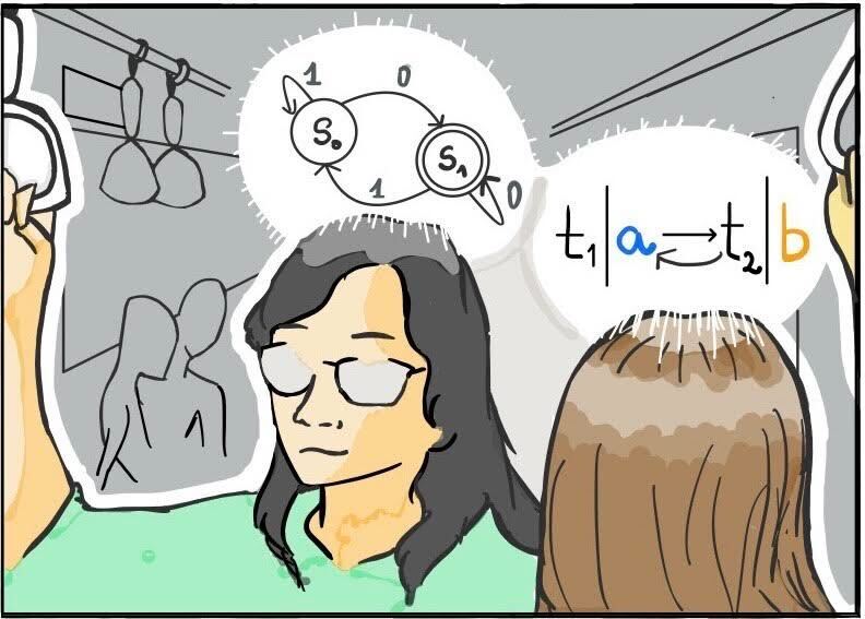
State transition systems are a pervasive object in theoretical computer science. Consider a deterministic finite automaton. The usual textbook definition (see, for example, “Automata and Computability” by Dexter Kozen) of a DFA is a 5-tuple $(Q, \Sigma, \delta : Q \times \Sigma \to Q, F \subseteq Q, q_0 )$ consisting of finite set of states $Q$, an alphabet $\Sigma$, a transition function $\delta : Q \times \Sigma \to Q$, that when given a state $q \in Q$ and a letter $a \in \Sigma$, $\delta(q,a) \in Q$ yields a state that can be obtained by reading a letter $a$ from the alphabet in some state $q$. The subset $F \subseteq Q$ describes a set of states which are accepting and $q_0$ denotes the initial state. The set of words over an alphabet $\Sigma$, which we denote by $\Sigma^{\ast}$ is the least set satisfying the following $$\epsilon \in \Sigma^{\ast} \quad \text{(Empty word } \epsilon \text{ is a word)}$$ $$\text{If }\; a \in \Sigma \;\text{and }\; w \in \Sigma^{\ast} \;\text{then}\; aw \in \Sigma^{\ast} \text{(Concatenating a letter to a word yields a word)}$$

We can now extend the transition function to operate on words. Define $\hat{\delta}: Q \times \Sigma^{\ast} \to Q$ by induction, using the construction of a word: $$\hat{\delta}(q,\epsilon) = q \quad\quad$$ $$\hat{\delta}(q, aw) = \hat\delta(\delta(q,a),w)$$

A word $w$ is accepted by the automaton if $\hat{\delta}(q_0, w) \in F$. The set of all accepted words $\{w \in \Sigma^\ast \mid \hat\delta(q_0,w) \in F\} \in 2^{\Sigma^\ast}$ is called the language of an automaton. The languages that can be accepted by a deterministic automaton with finitely many states are called regular or rational languages.

Now, let’s slightly relax and rearrange the definitions.

First, let’s drop the idea having an initial state. Instead of the language of the automaton, we will now speak of a language $q \in Q$ of a state of an automaton. Every automaton induces a function $\dagger : Q \to 2^{\Sigma^{\ast}}$ which is given by $q \mapsto \{ w \in \Sigma^\star \mid \hat\delta(q,w) \in F\}$, and the set $\dagger(q)$ is called the language of the state $q$.

We can view the set of accepting states, as a function $o : Q \to 2$ to the two-element set, such that $o(q)=1 \Leftrightarrow q \in F$. Currying the transition function yields $\delta : Q \to Q^\Sigma$. Now, we can use cartesian product and combine the functions $o$ and $\delta$ into a function $\langle o, \delta\rangle : Q \to 2 \times Q^\Sigma$. Intuitively, such function takes a state to its one-step observable behaviour. Finally, we will drop the requirement of the set of states to be finite. Automata with infinitely many states can denote more expressive langauges from the Chomsky hierarchy, such as Context-Free Languages.

Each deterministic automaton can be now viewed as a pair $(Q, \alpha : Q \to 2 \times Q^\Sigma)$. More interestingly, we can endow the set of all languages $2^{\Sigma^{\ast}}$ with the structure of a deterministic automaton. Define the acceptance function $\epsilon ? : 2^{\Sigma^{\ast}} \to 2$ to be given by $\epsilon ? (L) = 1 \Leftrightarrow \epsilon \in L$. In other words, a language will be an accepting state if and only if it contains the empty word. Now, define a transition function $(-)_a : 2^{\Sigma^{\ast}} \times \Sigma \to {2^{\Sigma^{\ast}}}$ to be given by $(L)_a=\{w \mid aw \in L\}$. Intuitively given a language $L$ and a letter $a$, we transition to a language obtained by cutting that letter from words that start with $a$ in the original language. The transition structure $\langle \epsilon ? , (-)_a \rangle$ is often called the semantic Brzozowski derivative, and the automaton $2^{\Sigma^{\ast}} \to 2\times (2^{\Sigma^{\ast}})^\Sigma$ is called the (semantic) Brzozowski automaton.

It can be observed that the Brzozowski automaton provides a form of a universal automaton in which every other deterministic automaton embeds in a well-behaved way. By well-behaved, we mean the following: - if a state $q\in Q$ in some automaton accepts, then its language $\dagger(q)$ contains an empty word, and so the language is an accepting state in the Brzozowski automaton, - if a state transitions to an another state on some letter $a\in \Sigma$, then in the Brzozowski automaton, the language of the first state transitions to the language of the second state on the same letter $a$.

Formally speaking, let $\langle o , \delta \rangle : Q \to 2 \times Q^\Sigma$ be a deterministic automaton with $Q$ being the set of states. The function $\dagger_{\langle o,\delta\rangle} : Q \to 2^{\Sigma^{\ast}}$ taking each state to its language satisfies the following for all $q \in Q$: - $o(q)=\epsilon?(\dagger_{\langle o,\delta\rangle}(q))$, - for all $a \in \Sigma$, $\left(\dagger_{\langle o,\delta\rangle}(q)\right)_a=\dagger_{\langle o,\delta\rangle}\left(\delta(a,q)\right)$.

In other words, the map $\dagger_{\langle o, \delta\rangle}$ to the Brzozowski automaton is structure-preserving. More generally, functions between any two deterministic automata satisfying the condition above are called homomorphisms. One can easily show that the Brzozowski automaton satisfies a certain universal property, namely that every other deterministic automaton admits a unique homomorphism to it (which is precisely the map which assigns to a state its language). We can use the Brzozowski automaton and language-assigining map to talk about the behaviour of states – we will say that two states are behaviourally equivalent if they are mapped to the same language in the Brzozowski automaton.

To sum up, the set of languages equipped with an automaton structure provides a universal and fully abstract treatment of the behaviours of states of deterministic automata.

Now, consider a different object of study within theoretical computer science and logic: Kripke frames. The usual way one gives the semantics of modal logic is through Kripke frames. A Kripke frame is a pair $(W, R \subseteq W \times W)$ consisting of a set of worlds $W$ and an accessibility relation $R \subseteq W \times W$. A valuation $v : W \to \mathcal{P}({AP})$ is a function, which assigns to each world a set of atomic propositions which are true in it. A Kripke frame along with a valuation forms a Kripke model. Given two Kripke models $((W_1, R_1 \subseteq W_1 \times W_1), v_1)$ and $((W_2, R_2 \subseteq W_2 \times W_2), v_2)$, we call a map $f : W_1 \to W_2$ a $p$-morphism if the following conditions hold: - if $u R_1 v$, then $f(u) R_2 f(v)$, - if $s R_2 t$ for some $s = f(u)$, then $u R_1 w$ and $t=f(w)$ for some $w \in W_1$, - $p \in v(w)$ if and only if $p \in v(f(w))$. domae $p$-morphisms are well-behaved morphisms preserving the structure of Kripke models (and hence the validity of modal formulae), and are thus somewhat similar in spirit to the homomorphisms between deterministic automata.

Observe that an accessibility relation $R \subseteq W \times W$ on a set of worlds can be viewed equivalently as a function $W \to \mathcal{P}(W)$. Similarly to deterministic automata, we can use the Cartesian product to combine seuthe accessibility relation and the valuation in a frame into a function $\langle R,v\rangle:W \to \mathcal{P}(W) \times \mathcal{P}({AP})$ which takes a world to its one-step observable behaviour. A Kripke model then becomes a pair $(W, \alpha : W \to \mathcal{P}(W) \times \mathcal{P}(AP))$.

Both deterministic automata and Kripke frames are pairs consisting of a set of states, and a one-step transition function which takes a state into some set-theoretic construction describing its bservable behaviour. These set-theoretic constructions are endofunctors $\mathsf{Set} \to \mathsf{Set}$, in our case $2 \times (-)^\Sigma$ and $\mathcal{P}(-) \times \mathcal{P}(AP)$. Deterministic automata and Kripke frames are concrete instances of coalgebras for an endofunctor.

Let’s spell out the concrete definitions.

Let $F : \mathcal{C} \to \mathcal{C}$ be an endofunctor on some category. An $F$-coalgebra is a pair $(X, \alpha : X \to F X)$ consisting of an object $X$ of category $\mathcal{C}$ and an arrow $\alpha : X \to F X$.

A homomorphism from $F$-coalgebra $(X, \beta)$ to $(Y, \gamma)$ is a map $f: X \to Y$ satisfying $\gamma \circ f = Ff \circ \beta$. Homomorphisms of deterministic automata and $p$-morphisms are the concrete instatiations of this definition.

Coalgebras and their homomorphisms form a category. Under an approriate size restrictions on the functor $F$, there exists a final coalgebra $(\nu F, t)$, which is a final object in the category of coalgebras. In other words, it satisfies the universal property that for every $F$-coalgebra $(X,\beta)$ there exists a unique homomorphism $\dagger \beta : X \to \nu F$. Final coalgebras provide a abstract domain providing denotation of the behaviour of $F$-coalgebras. We already saw that in the case of deterministic automata, Brzozowski automaton provided a final coalgebra, where formal langauges denoted the behaviour of states of automata. Finally, the concrete notion of behavioural equivalence was given by language equivalence.

Behavioural equivalence of quantitative systems

Having introduced the motivation for the study of coalgebras, we move on to a particular example, which will motivate looking at behavioural distance. Consider an endofunctor $\mathcal{D} : \mathsf{Set} \to \mathsf{Set}$, which takes each set $X$ to the set $\mathcal{D} X = \{\mu : X \to [0,1] \mid \sum_{x \in X} \mu(X) = 1\}$ of discrete probability distributions over $X$. On arrows $f : X \to Y$, we have that $\mathcal{D} f : \mathcal{D}X \to \mathcal{D}Y$ is given by $\mathcal{D} f (\mu)(y) = \sum_{f(x) = y} \mu(x)$, also known as the pushforward measure. Coalgebras for $\mathcal{D}$ are precisely Discrete Time Markov chains. Since all the states in such a case have no extra observable behaviour besides the transition probability, it turns out that all the states are behaviourally equivalent. Let’s consider a slightly more involved example, where each state can also be terminating with some probability.

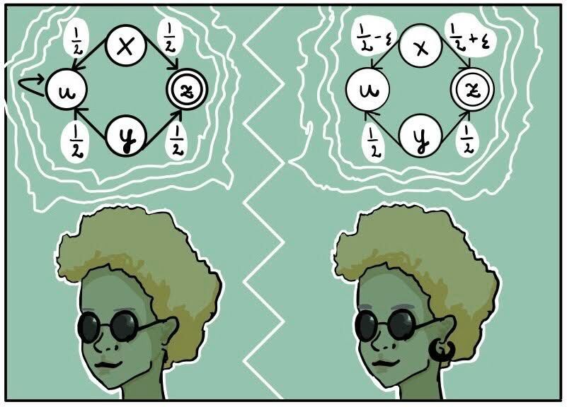
Consider a composite functor $\mathcal{D}(1 + (-))$ that takes a set $X$ to $\mathcal{D}(\{\ast\}\cup X):=\mathcal{D}(1+X)$. Coalgebras for it can be thought of Markov Chains with potential deadlock behaviour. Now, let’s look at a concrete example of a four state automaton

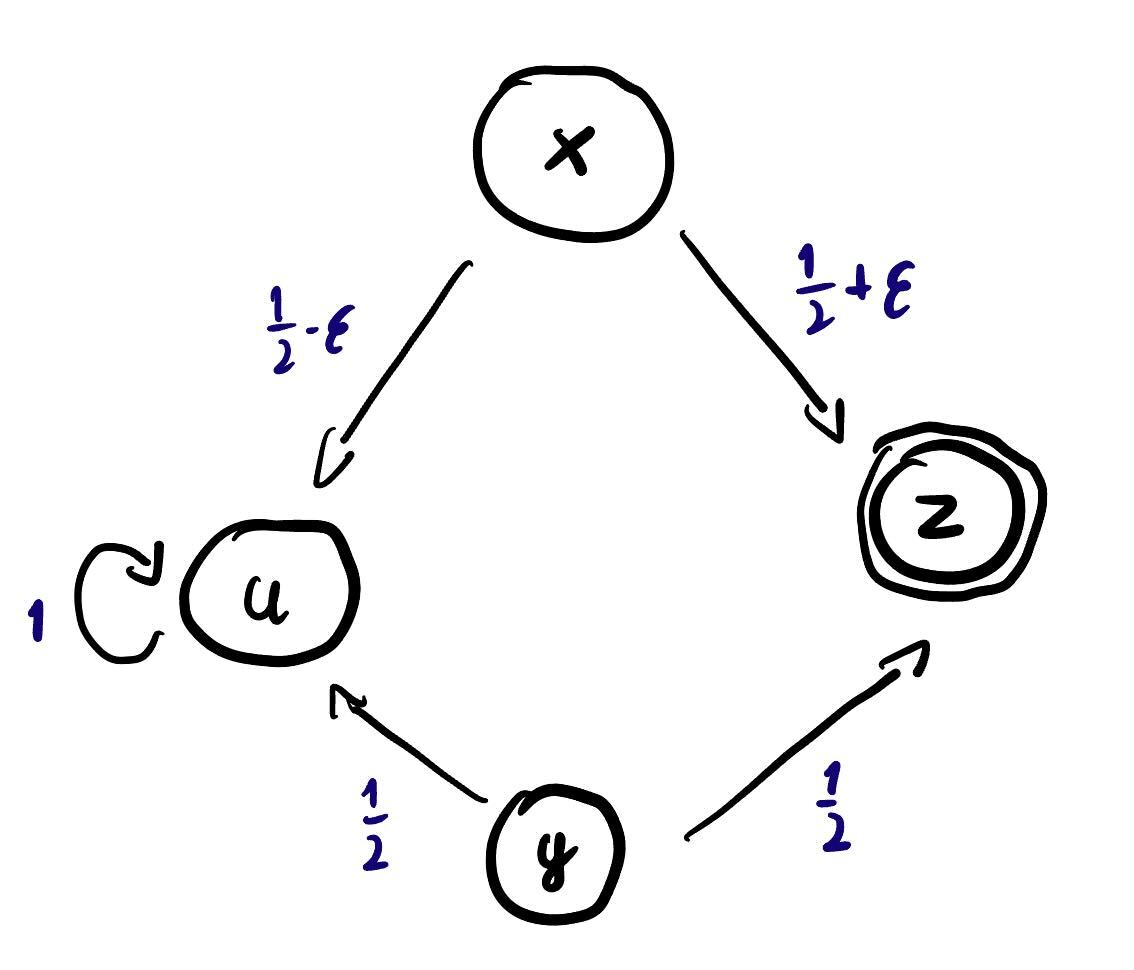
State $z$ enters deadlock with probability $1$, while state $u$ has a self loop with probability $1$. The functor $\mathcal{D}(1 + (-))$ admits a final coalgebra and it is not too hard to observe that states $u$ and $z$ exhibit completely different behaviour and will be mapped into distinct elements of the carrier of final coalgebra. State $y$ has $\frac{1}{2}$ probability of ending in $u$ and $\frac{1}{2}$ probability of ending in $z$. It has two equiprobable options of tranisitioning to states, which behave in a different way from eachother. It is not too hard that $y$ is also not behaviourally equivalent to $u$ and $z$. Finally, consider the state $z$. Let $\epsilon \in [0, \frac{1}{2}]$. State $x$ can transition to $u$ with probability $\frac{1}{2} - \epsilon$ and transition to $z$ with probability $\frac{1}{2} + \epsilon$. Observe that only when $\epsilon=0$ state $x$ is behaviourally equivalent to $y$. Even for very small non-zero values of $\epsilon$, states $x$ and $y$ would be considered inequivalent.

For practical purposes, coalgebraic behavioural equivalence (for coalgebras on $\mathsf{Set}$) might be way too restrictive. In the case of systems exposing quantitative effects, it would be more desirable to consider a more robust notion of behavioural distance, which would quantify how similarly two states behave. The abstract idea of distance has been captured by mathematical notion of metric spaces and related objects.

Pseudometrics and $\mathsf{PMet}$

Underlying the behavioural distance between states of a coalgebra is the mathematical idea of distance. Most commonly, distance is treated in the form of a metric space. A metric space is a set $X$ with a distance function $d:X\times X\to [0,\infty)$ that satisfies the following axioms for each $x,y\in X$. - Separation: $d(x,y)=0\iff x=y$. - Symmetry: $d(x,y)=d(y,x)$, - Triangle inequality: $d(x,z)\leq d(x,y)+d(y,z)$.

In the context of coalgebras, however, we may wish to have a slightly altered notion of distance to capture behavioural similarity.

If two states behave identically, then even if they are not the same state, we expect their distance to be zero. Thus, we relax the separation axiom and only require that $d(x,x)=0$ for all $x\in X$. This yields a pseudometric. Note that a pseudometric is still symmetric and still fulfills the triangle inequality. It is also possible to have an asymmetric notion of distance, where both separation and symmetry are relaxed. The distance function obtained like that is a function $d:X\times X\to [0,\infty)$ that only fulfills the triangle inequality, but it is possible that $d(x,y)=0$ and $d(x,y)\neq d(y,x)$ for some $x\neq y$. This is called a hemimetric, and it occurs when formalising distance via fuzzy lax extensions.

Finally, we may wish to bound the distance, to have a way of expressing when two states are “maximally different”. For example, we use this to express that an accepting and a non-accepting state are maximally different. In order to accommodate that, we instead define the distance function as $d:X\times X\to [0,\top]$, where $\top \in (0,\infty]$. In the context of behavioural distances on coalgebra, it is common to take $\top = 1$ or $\top = \infty$. However, in the case of $\top = \infty$, this requires a way of calculating with infinity, and this is resolved by defining distance and addition with infinity as $$d(x,\infty) = \infty,\: x\neq \infty; \quad d(\infty,\infty)=0;\quad x+ \infty = \infty,\: x\in [0,\infty].$$

Once we fix the bound $\top$ and some set $X$, we can consider the set $\mathsf{PMet}(X)$ of all pseudometrics $d$ over $X$. It turns out that under the pointwise order and appropriate definitions of meet and join, $\mathsf{PMet}(X)$ becomes a lattice. In particular, the order is given by $$d_1 \leq d_2 \iff d_1(x,y)\leq d_2(x,y) \quad\forall x,y\in X,$$ and for a subset $D\subseteq \mathsf{PMet}(X)$, $$(\sup D)(x,y) := \sup \{d(x,y)\mid d\in D\},\quad\inf D := \sup \{d\mid d \in \mathsf{PMet}(X) \land \forall d'\in D. d\leq d'\}.$$

Moreover, it is a complete lattice, meaning each subset has a meet and a join. The lattice being complete implies that the category of all pseudometric spaces for a fixed $\top$ is complete and cocomplete, which in turn implies that the category has products and coproducts.

Here’s how we define this category of pseudometric spaces:

The category $\mathsf{PMet}$ for a fixed $\top\in (0,\infty]$ has - pseudometric spaces $(X,d_X)$ as objects, - nonexpansive maps $f:(X,d_X)\to (Y,d_Y)$ as morphisms.

The definition of nonexpansive maps is quite immediate: $$d(f(x),f(y))\leq d(x,y)\quad \forall x,y\in X,$$ i.e. the maps do not increase distances between elements. Clearly, the composition of nonexpansive maps is nonexpansive as well, and the identity map is nonexpansive.

Motivation from transportation theory

In the long run, we would like to be able to go from distances on the states of coalgebra to distances on observable behaviours. For now, let’s focus our attention on the discrete distributions functor. Let $X$ be a set equipped with a $\top$-pseudometric structure on it, given by $d_X : X \times X \to [0, \top]$ and let’s say we have two distributions $\nu, \mu \in \mathcal{D}X$. We would like define a pseudometric structure $d_{\mathcal{D} X} : \mathcal{D}X \times \mathcal{D}X \to [0,\top]$ which would allow us to calculate the distance between $\nu$ and $\mu$.

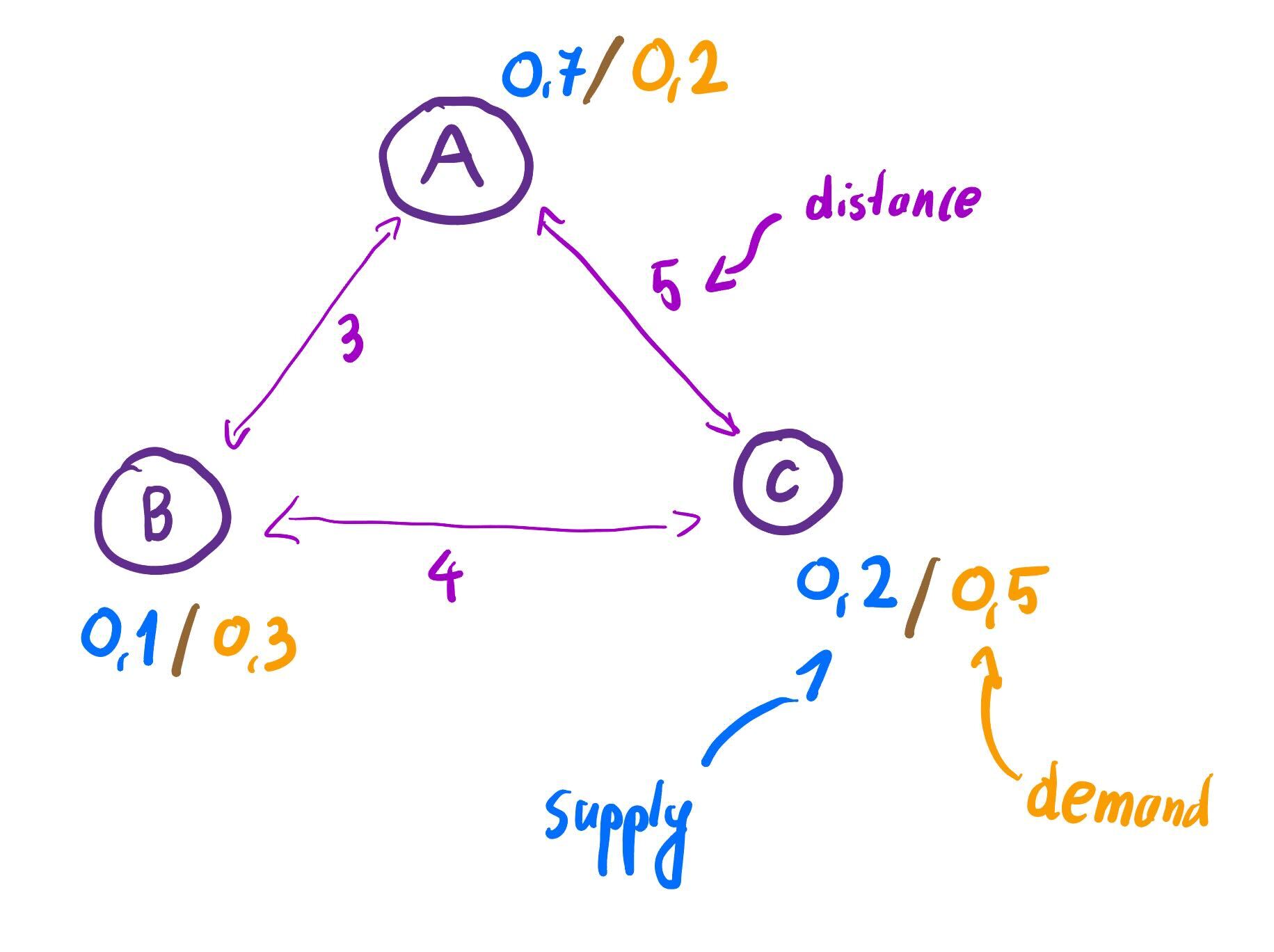
It turns out, there is well-known answer to this question, coming from the field of transportation theory. Let’s make the example slightly more concrete. Let $X = \{A,B,C\}$ and from now on we will omit the subscript on the map $d_X :X \times X \to [0,\top]$

Imagine that $A, B$ and $C$ are three bakeries with an adjacent shop where one can taste the pastries. We have that $d(A,A)=d(B,B)=d(C,C)=0$. Moreover, let’s say that distance between $A$ and $B$ is three ($d(A,B)=d(B,A)=3$), while $B$ and $C$ are in distance four ($d(B,C)=d(C,B)=4$) and $A$ and $C$ are in distance five ($d(A,C)=d(C,A)=5$). Hence, $d$ is a metric space.

Let $\nu \in \mathcal{D} X$ be the distribution of supply of the pastries in each of the bakeries. $\nu(A) = 0.7$, $\nu(B)=0.1$ and $\nu(C)=0.2$

Let $\mu \in \mathcal{D} X$ be the distribution of demand in pastry shops adjactent by the bakeries. We have that $\mu(A) = 0.2$, $\mu(B)=0.3$ and $\mu(C)=0.5$.

In bakery $A$, there are more pastries produced than being consumed, while in $B, C$ more people are having their pastry than $B, C$ can actually produce. The reasonable thing to do for an owner of these places, would be to redistribute the pastries so the needs of customers are satisfied. One way of solving this problem would be to come up with a transport plan, a map $t : X \times X \to [0,1]$, where $t(x,y) = k$ would intuitively mean move the ratio of $k$ pastries from bakery $x$ to $y$. Such a transport plan should satisfy

• For all $x \in X$, $\nu(x) = \sum_{x' \in X} t(x,x')$ - whole supply of pastries is used
• For all $x \in X$, $\mu(x) = \sum_{x ' \in X'} t(x',x)$ - all demand is satisfied

In other words, one can think of $t : X \times X \to [0,1]$ as a joint probability distribution $t \in \mathcal{D}(X \times X)$ which can be marginalised into $\nu$ and $\eta$. Such a joint distribution, which equivalently describes a transportation plan is called a coupling of $\eta$ and $\mu$. There can be multiple transportation plans, but some might involve unnecessary movement of pastries to the bakery which is too far away. Each transportation plan can be assigned a cost, proportional to the distance that each fraction of pastries needs to travel. The cost of plan $t$ is given by $c_t$ defined as $$c_t = \sum_{(x,y) \in X \times X} d(x,y)t(x,y)$$

Let $\Gamma(\nu, \mu)$ denote the set of all couplings of $\nu$ and $\mu$. The owner of the bakeries is aiming to minimise the total cost of transportation. The minimal cost of the tranportation from $\mu$ to $\nu$ is given by the following $$d^{\mathcal{D}\downarrow}(\mu, \nu) = \min\{\sum_{(x,y) \in X \times X} d(x,y)t(x,y) \mid t \in \Gamma(\nu, \mu)\}$$

It turns out that phrasing this minimisation problem as a linear program guarantees existence of the optimal coupling, which costs the least. The definition above actually defines takes a pseudometric $d : X \times X \to [0, \top]$ and transforms it into a pseudometric $d^{\mathcal{D}\downarrow} : \mathcal{D} X \times \mathcal{D} X \to [0, \top]$ on distributions over $X$. This (pseudo)metric is known as Wasserstein metric.

In our example, it turns out that the most cost optimal plan is to do the following: - Move $\frac{1}{5}$ of pastries from $A$ (where there is an overproduction) to $B$ - Move $\frac{3}{10}$ of pastries from $A$ (where there is an overproduction) to $C$

The optimal cost is given by the following $$d^{\mathcal{D}\downarrow}(\nu,\mu)= \frac{1}{5}\cdot 3 +\frac{3} {10} \cdot 5 = 2.1$$

Now, consider an alternative approach. Let’s say that instead of organising transport on their own, the owner of the bakery will hire an external company to do that. In such a setting the company will assign to each bakery a price for which it buy pastries (in case of overproduction) or sells (in the case of higher demand). Formally it will be modelled as functions $$f : X \to \mathbb{R}^{+}$$ satisfying that for all $x,y \in X$, we have that $$\mid f(x) - f(y)\mid \leq d(x,y)$$ One can think of the requirement above that intuitively owner of the bakeries won’t accept situation when they have to pay more for the transport than when performing the transport on their own. Formally speaking, it means that $f$ is a nonexpansive function from $(X,d)$ to nonnegative reals equipped with euclidean norm $d_e$. Given a price plan $f : X \to \mathbb{R}^+$ the income of the company will be given by $$\sum_{x \in X} f(x) (\mu(x) - \nu(x))$$

The external company would like to maximise their profits, so the optimal profit would be given by $$d^{\uparrow \mathcal{D}}(\mu, \nu)= \sup\left\{ \sum_{x \in X}f(x)(\mu(x)-\nu(x)) \mid f : (X, d) \to (\mathcal{R}^{+}, d_e) \text{ nonexpansive}\right\}$$

The optimal pricing plan exists (again by formulation of the problem as the linear programming problem), so the above is well-defined. $d^{\mathcal{D}\uparrow}$ happens to be a pseudometric, as long as $d$ is. This notation of distance between distributions is known as Kantorovich metric.

For the example above, the optimal price plan is given by the following: - Owner of the bakeries gives out the excess from $A$ for free ($f(A)=0$) - Bakery $B$ buys necessary pastries for three monetary units ($f(B)=3$) - Bakery $C$ does the same with the cost of five units ($f(C)=5$) In such a case, the distance is given by the following $$d^{\mathcal{D}\uparrow}(\mu, \nu) = 0 \cdot (0.2-0.7) + 3 \cdot (0.3 - 0.1) + 5 \cdot (0.5 - 0.2)= 2.1$$

In this particular case, we ended up with the same distance as before, when talking about transport plans. It is no coindidence and actually an instance of the quite famous result, know as Kantorovich-Rubinstein duality. We have that $$d^{\mathcal{D}\uparrow}=d^{\mathcal{D}\downarrow}$$ One can intuitively think that minimising the transportation cost is dual to the external company trying to maximise their profit.

Liftings to $\mathsf{PMet}$

The above distances can also be thought of as answers to the following lifting problem. If $F$ is a functor on $\mathsf{Set}$, then how can one construct a functor $\overline{F}$ on $\mathsf{PMet}$ such that

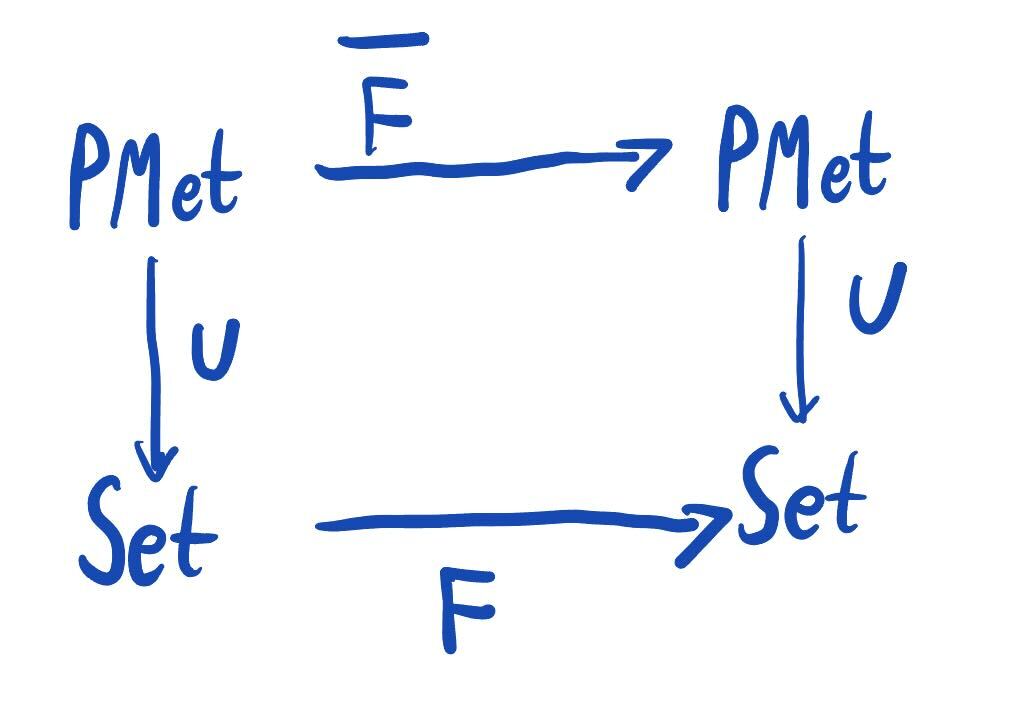
commutes? In other words, how can we construct a functor $\overline{F}:\mathsf{PMet}\to \mathsf{PMet}$ that acts as $F$ on the underlying sets and nonexpansive functions?

The first priority when defining a lift is that $\overline{F}$ should be a functor. That is, when given a pseudometric space $(X,d)$, we need to define a pseudometric on $FX$ in a sensible way. Since the definition of a lift implies that $\overline{F}f$ is just $Ff$ for all nonexpansive $f:(X,d_X)\to (Y,d_Y)$ and we need $Ff$ to be nonexpansive, then the pseudometrics on the objects $FX$ and $FY$ need to ensure that $Ff$ is nonexpansive. Then and only then does $\overline{F}$ become a functor.

Put precisely, in order to have a lift, we require that - for any pseudometric space $(X,d_X)$, we have a pseudometric space $(FX,d_X^F)$ such that - for any nonexpansive functions $f:(X,d_X)\to (Y,d_Y)$, the function $Ff:(FX,d_X^F)$ and $(FY,d_Y^F)$ is nonexpansive.

In the above case of the distance between two distributions, an initial distance $d_X$ between elements of $X$ was given, and the distance on $\mathcal{D}X$ was defined. The functoriality of such a construction was not checked, but it holds (and the proof in the abstract case can be found in the referential paper).

Inspired by the constructions in the case of $\mathcal{D}$, Kantorovich and Wasserstein liftings can be defined for arbitrary functors. This is also where the relevance to coalgebras becomes evident – the notion of a lift enables us to start with a pseudometric on the state space $X$, and induce from that a pseudometric on the space of possible behaviours $FX$.

In the mechanics of lifting a pseudometric, it is useful to consider an evaluation function: a function $ev_F:FX\to [0,\top]$ for all objects $X$. Then, we can consider the function $\widetilde{F}f:FX\to [0,\top]$ defined as $\widetilde{F}f = ev_F\circ Ff$ for morphisms $f:X\to[0,\top]$. Certain choices of evaluation functions may arise in the case of particular functors. For example, in the case of $\mathcal{D}$, the evaluation function $\mathcal{D}X\to [0,1]$ is taken to be the expected value $\mathbb{E}(-)$.

Kantorovich lifting

The Kantorovich lifting is defined as follows. Let $F$ be a functor on $\mathsf{Set}$ with an evaluation function $ev_F$. Then the Kantorovich lifting is the functor $\overline{F}$ that takes $(X,d)$ to the space $(FX,d^{\uparrow F})$, where $$d^{\uparrow F}(t_1,t_2) := \sup\{\: d_e\left( \widetilde{F}f(t_1),\widetilde{F}f(t_2)\right)\:\mid\: f:(X,d)\to ([0,\top],d_e) \:\}.$$

This is in fact the smallest possible pseudometric that makes all functions $\widetilde{F}f:FX\to [0,\top]$ nonexpansive. The Kantorovich lifting preserves isometries.

Wasserstein lifting

The Wasserstein distance $d^{\downarrow F}$ that is required to define the Wasserstein lifting, needs more work to set up. Altogether, it requires a generalised definition of couplings, some well-behavedness conditions from the evaluation function, and the preservation of weak pullbacks from the functor.