Mixed Volume
Posted by Tom Leinster
.")
Take convex bodies in , or convex bodies in , or, more generally, convex bodies in . Mixed volume assigns to each such family a single real number.
The mixed volume of convex bodies is written as , and it’s uniquely characterized by the following three properties:
- Volume: , for any convex body
- Symmetry: is symmetric in its arguments
- Multiadditivity: equals for any convex bodies and , where denotes Minkowski sum.
This looks rather like the characterization of determinant: is unique satisfying , antisymmetry, and multilinearity. One difference is that we have symmetry rather than antisymmetry. But a much bigger difference is that where determinant assigns a number to vectors in , mixed volume assigns a number to convex bodies in .
But maybe you don’t find the unique characterization satisfying. What is mixed volume?
First I should be precise about what I mean by ‘convex body’. I simply mean a compact, convex, nonempty subset of . (Often people include the condition that the interior is nonempty, but I’m not requiring that.) You might raise an eyebrow at the word ‘nonempty’, but it really does matter.
In a moment I’ll give you lots of examples of mixed volume. Later on, I’ll give you the definition, and I’ll also list some of the other properties that it satisfies (apart from the three that characterize it uniquely). But the examples will be easier to understand if I tell you one of those properties right now:
4. Translation-invariance in each coordinate: for any convex bodies and any .
Since is symmetric, this implies that
In other words, sliding the bodies around doesn’t change the mixed volume. (Changing their orientations usually does, as we’ll see.) Knowing this helps us to speak more freely. If, say, , then I can say ‘let be a rectangle with edges parallel to the coordinate axes’ — I don’t need to say where in the plane it lives.
Examples of mixed volume
Example I’ve already mentioned that for any convex body . Now suppose that our convex bodies are not necessarily equal, but are all scalings of one another. Given a convex body and scalars , we have
where means . To put it another way: if are all scalings of one another then
Example The previous example is misleading, because it doesn’t reveal that in general, mixed volume depends on how the convex bodies interact with one another. But a simple example with will show this. Let be an rectangle and a rectangle, both with their edges parallel to the coordinate axes. Then
Here’s a picture:
The mixed volume — which for could be called ‘mixed area’ — is not derived from the areas of and , shown in grey. Instead, it’s the (arithmetic) mean of the areas of the two red rectangles.
The formula for looks a bit like the determinant formula …. We’ll come back to this.

Example Let’s generalize the previous example to higher dimensions. Rectangles, then, will become cuboids. Previously we established that the word ‘cuboid’ is known to British schoolchildren and comedians, but not American math professors (I’m teasing, John). I believe American English uses some quaint term such as ‘orthogonal parallelepiped’. Anyway: let be any natural number, let be an matrix of nonnegative reals, and for , let
(Or you could take to be a translate of this; it doesn’t matter.) Then
Again, this can usefully be compared to the determinant formula
Apart from the constant factor, the only difference is in the signs. This corresponds to mixed volume being symmetric and determinant being antisymmetric.
I said before that whereas determinant assigns a number to any vectors in , mixed volume assigns a number to any convex bodies in . Actually, every vector gives rise to a convex body: it’s the axis-parallel cuboid whose long diagonal is . For example, the vector gives rise in this way to the cuboid . In the last paragraph, we compared the determinant of the vectors with the mixed volume of the convex bodies they give rise to.
Minkowski’s theorem
I still haven’t told you the definition of mixed volume. One reason why not is that in order to even state the definition, we first need to know the following theorem of Minkowski.
Theorem (Minkowski) Let and be natural numbers. Fix convex bodies in . Then the function
() is a polynomial, homogeneous of degree .
If you understand Minkowski’s theorem, you understand mixed volume. So I’ll do my best to explain it.
The first thing to notice is that whereas we had been discussing bodies in -dimensional space, we’re now discussing bodies in -dimensional space. Of course, you can take , but it’s probably easier to understand Minkowski’s theorem if we treat it at its natural level of generality.
Now let’s look for the first nontrivial case.
For , the theorem is trivial.
For , it says that given any convex body in , the function
() is a polynomial in , homogeneous of degree . That’s true, and doesn’t even use convexity: the polynomial is .
It’s when that things start to get interesting. The statement is that for convex bodies , the function
is a homogeneous polynomial of degree . Because itself is homogeneous of degree , we might as well fix to be . Then Minkowski is telling us that
is a polynomial of degree .
Why is that so? The picture below shows an example with . Here is the blue quadrilateral, is any one of the green egg shapes, and is the whole thing, including the grey parts. (The four copies of that I’ve chosen to draw are for the four vertices of .)
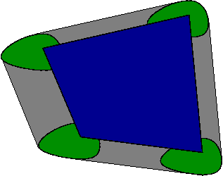
Minkowski’s theorem implies that the area of the whole thing is a (possibly degenerate) quadratic in .
So let’s try to understand some special cases. I’m sticking with : that is, I’m trying to explain why is a polynomial in of degree at most , whenever and are convex bodies in .
Example Take to be a singleton . Then , a translate of . Hence for all . This is certainly a polynomial in of degree .
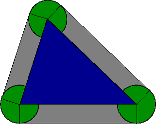
Example Take . Then
which is indeed a polynomial of degree .
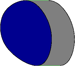
Example Choose a point and take to be the straight line segment from to . Then
Here’s a picture with and with somewhere on the positive -axis:
As before, is in blue. It’s clear that the area of the grey part is proportional to the horizontal distance over which has been smeared out — that is, proportional to . This gives
for some constant , and again, this is a polynomial in of degree .
Example Take to be the unit ball. Then is the closed -neighbourhood of , that is, the set of all points such that . And there’s a famous theorem giving the volume of the -neighbourhood: Steiner’s theorem.
By law, every explanation of Steiner’s theorem must contain the following diagram:
Staring at this picture should reveal to you the following truth: for convex bodies in ,
This is a polynomial in of degree . There’s a similar formula in higher dimensions. The coefficients are, up to a constant factor, the intrinsic volumes of .
That’s enough explanation; it’s time to give you the definition.
The definition of mixed volume
Take convex bodies in , say . Minkowski’s theorem states that
is a polynomial in , homogeneous of degree . The mixed volume is the coefficient of in this polynomial, divided by .
This definition is apt to look mysterious. For a start, why this particular coefficient? It’s because, as it turns out, mixed volume tells you all the coefficients.
The precise statement is as follows. Take any natural numbers and , and any convex bodies in . Then
So if someone put an implant in your brain that enabled you to calculate any mixed volume, you’d also be able to calculate the Minkowski polynomial of any family of convex bodies.
Example Take . Then this tells us that
But , so what this essentially says is that
You can check this in some of the examples above.
Another way to express this equation is:
Here is the multinomial coefficient , and by definition,
where each appears times. So, mixed volumes with repeated arguments are important. In this respect, mixed volume is unlike determinant: because of antisymmetry, determinants with repeated arguments are trivial.
The unique characterization
I began by stating that mixed volume is uniquely characterized by three properties: the volume property (), symmetry, and multiadditivity. It’s easy to prove that when , there’s at most one function satisfying the three properties. It’s a bit like the proof that in an inner product space, the norm determines the inner product. Indeed, if satisfies the properties then by multiadditivity we have
and so by symmetry and the volume property,
(This is the same as the formula in the last example, rearranged and with .) So mixed volume can be expressed in terms of ordinary volume and Minkowski sums.
You can do the same kind of thing in higher dimensions. When , for instance, you get
The formula for general is now exactly as you’d guess.
That’s a very explicit formula for mixed volume, though it’s not clear that it gives much insight. By way of analogy, does the formula
give you a lot of insight into multiplication of real numbers? It’s probably important in some contexts, and it’s interesting that multiplication can be built out of addition, squaring and halving. But it’s not how most of us think about multiplication.
Further properties of mixed volume
In the absence of a single really compelling way to understand mixed volume, I’ve described several ways in which it can be half-understood. There’s the unique characterization by three properties, there’s the analogy with determinants, there are examples, there’s the definition in terms of the polynomial in Minkowski’s theorem, and there’s the formula we just met, giving mixed volume as a linear combination of ordinary volumes.
I’ll finish with another way of half-understanding it. It’s a long list of properties that mixed volume satisfies. For completeness, I’ll begin with the four that we’ve already seen.
- Volume:
- Symmetry: is symmetric in its arguments
- Multiadditivity:
- Translation-invariance in each coordinate:
- Isometry-invariance: for any in the isometry group of
- Special linear invariance: for any
- Scaling: for any
- Singletons:
- Monotonicity: whenever
- Nonnegativity:
- Continuity: is continuous with respect to the Hausdorff metric on convex bodies
- Valuation in each coordinate: as long as is convex.
Perhaps mixed volume can be summarized as a mutual measure of size. The properties listed all fit well with this description. For example, the last one says that coordinatewise, mixed volume is a valuation or finitely additive measure. The analogy between mixed volume and determinants points in the same direction: the determinant of vectors in is, after all, the volume of the parallelepiped that they generate. But the direct geometric significance of mixed volume remains, to me, elusive.
Re: Mixed Volume
I’ll add a puzzle.
I described the analogy between mixed volume and determinant. Now, in linear algebra, the determinant of an operator is often best thought of as the product of its eigenvalues, taken with their algebraic multiplicities. But the spectrum — that is, the set-with-multiplicities of eigenvalues — is really a more fundamental object than the determinant. What is the analogue of the spectrum in the world of convex bodies?
I don’t know the answer.