The n-Category Café

[Remember that throughout this post we have $n=2m-1$ is an odd positive integer.]

The work of Meckes and Barceló-Carbery

As a reader of this blog you might well know that magnitude of finite metric spaces is usually defined using weightings. Mark Meckes showed that the natural extension of magnitude to infinite subsets of Euclidean space can be defined using potential functions.

Before going anywhere, however, recall that the Laplacian operator $\Delta$ is the differential operator on functions on $\mathbb{R}^n$ given by $\Delta f=\sum_{i=1}^n \frac{\partial ^2f}{\partial x_i^2}$.

Now, for $X$ a compact subset of $\mathbb{R}^n$ with smooth boundary, a potential function $h$ for $X$ is a function $h\colon \mathbb{R}^n\to \mathbb{R}$ with properties including the following:

• $h= 1$ on $X$;
• $(\id- \Delta)^m h = 0$ (weakly) on $\mathbb{R}^n\setminus X$;
• $h$ is $m-1$ times differentiable on $\mathbb{R}^n$, and the $m$th derivative exists in an $L^2$-sense;
• $h(x)\to 0$ as $x\to \infty$.

You can see an example below in the next section.

Barceló and Carbery built on the results of Meckes to show that for a compact convex domain $X$ in $\mathbb{R}^n$ with smooth boundary the following recipe can be used to calculate the magnitude of $X$.

First define $\mathcal{D}^i$ to be the order $i$ differential operator on the boundary by

$$\mathcal{D}^{2j}= \Delta^{j},\,\,\,\,\, \mathcal{D}^{2j+1}=\textstyle\frac{\partial}{\partial \nu}\Delta^{j},$$

where $\textstyle\frac{\partial}{\partial \nu}$ means the derivative in the normal direction to the boundary.

The Barceló-Carbery Recipe for Magnitude. Suppose $X\in \mathbb{R}^n$ is a compact domain with smooth boundary.

1. Find a solution $u\colon \mathbb{R}^n\setminus X\to \mathbb{R}$ with $u(x)\to 0$ as $x\to \infty$ of the differential equation $$(Id-\Delta)^m u=0\,\,\,\, \text{on}\,\,\mathbb{R}^n\setminus X$$ subject to the boundary conditions $$u=1,\, \mathcal{D}^1(u) =0,\, \mathcal{D}^2(u) =0,\, \dots, \mathcal{D}^{m-1}(u) =0, \,\,\,\, \text{on}\,\, \partial X.$$

2. The magnitude is then calculated by $$\text{mag}(X)=\frac{1}{n!\,\omega_n}\left(\text{vol}(X)+\sum_{m/2\lt j\le m}(-1)^j\binom{m}{j}\int_{\partial X} \mathcal{D}^{2j-1}(u)\,\mathrm{d}{s}\right).$$

Barcelo and Carbery actually stated their result for convex domains, but if we assume smoothness of the boundary then we can drop the convexity assumption.

The potential function $h$ of $X$ is related to the $u$ in the recipe by extending it to all of $\mathbb{R}^n$ by taking it to be $1$ on $X$.

Let’s have a look at a simple example that we’ll return to through this post.

A one-dimensional example

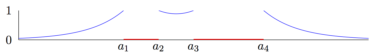
Consider the union of two intervals in the line: $X:=[a_1, a_2]\cup[a_3, a_4]\subset \mathbb{R}$ for $a_1\lt a_2\lt a_3 \lt a_4$. The differential equation to solve in the Barceló-Carbery recipe is then

$$u-u''=0 \,\,\,\, \text{on }\,\,\mathbb{R}\setminus X=(-\infty, a_1]\cup [a_2,a_3]\cup [a_4,\infty),$$

and the boundary conditions are

$$u(x)=1\,\,\,\,\text{for }\,\,x\in \{a_1, a_2, a_3, a_4\}.$$

This is easy to solve by hand and you find the solution

$$u(x)=\begin{cases} e^{-(a_1-x)} & x\in (-\infty, a_1], \\ (e^{-(x-a_2)}+e^{-(a_3-x)})/(e^{-(a_3-a_2)}+1) & x\in [a_2, a_3], \\ e^{-(x-a_4)} & x\in [a_4, \infty). \end{cases}$$

Here is the graph of the potential function.

Now according to Barceló and Carbery’s recipe we can calculate the magnitude as

$$\begin{aligned} \mathrm{mag}(X) & =\frac{1}{2}\left(\mathrm{vol}(X)-(-u'(a_1)+ u'(a_2)-u'(a_3)+u'(a_4))\right) \end{aligned}$$

But it is easy to compute from the formula for $u$ above that

$$u'(a_1)=1=-u'(a_4), \quad -u'(a_2)=\tanh\left(\frac{a_3-a_2}{2}\right)=u'(a_3)$$

and so

$$\begin{aligned} \mathrm{mag}(X)&=\tfrac{1}{2}(a_2-a_1+a_4-a_3)+1 +\tanh(\frac{a_3-a_2}{2}) \end{aligned}$$

which we can write as

$$\begin{aligned} \mathrm{mag}(X) &= \tfrac{1}{2}\mathrm{vol}(X)+\chi(X)-\frac{2}{\exp(a_3-a_2)+1}. \end{aligned}$$

A key point to note here is that to calculate the magnitude we don’t actually need to know the whole potential function $u$, we only need to know certain of its derivatives at the boundary. So we start with a differential equation, specify sufficiently many derivatives at the boundary to give a unique solution and then find values of other derivatives at the boundary. This is a process which is well studied in the area of boundary value problems and is embedded in the notion of the Dirichlet to Neummann operator which we now look at.

The Dirichlet to Neumann operator

As you surely know, when solving a differential equation, you impose boundary conditions in order to pin down the solution. You might impose different boundary conditions in different situations. For instance, the classical Dirichlet boundary conditions for a problem of second order fix the value of the function on the boundary, whereas the classical Neumann boundary conditions fix the normal derivative of the function on the boundary.

For the calculating magnitude, the boundary value problem is of order $2m$, not of order $2$. We think of the boundary conditions $f=1,\, \mathcal{D}^1(f) =0, \, \mathcal{D}^2(f) =0, \,\dots, \mathcal{D}^{m-1}(f) =0$, which involves derivatives of order $0$ up to $m-1$, as analogues of Dirichlet boundary conditions. To compute the magnitude we need to determine the derivatives of the solution of order $m$ up to $2m-1$, which we think of as analogues of Neumann boundary conditions.

Given Dirichlet boundary conditions we want to determine the corresponding Neumann boundary conditions. Let’s think what this means.

If you have a differential equation $L f =0$ on a domain $X$ then specifying the boundary condition means imposing a set of equations of the form

$$(\delta_1f)(x)=v_1(x),\,\,\dots,\,\,(\delta_p f)(x)=v_p(x), \,\, \text{for all }\,\,x\in \partial X$$

where each $\delta_i$ is a differential operator on the boundary $\partial X$ and each $v_i\in \mathrm{Fun}(\partial X)$ belongs to a suitable space of functions on the boundary. (We will avoid technicalities and complicated notation by using $Fun(\partial X)$ to stand for some space of functions, which might vary depending on context.)

When the boundary conditions give a unique solution to the differential equation – such as in the Barceló-Carbery Recipe – then for any other set $\{\tilde {\delta}_j\}_{j=1}^q$ of differential operators on the boundary there is a map, the Dirichlet to Neumann operator, between tuples of function on the boundary:

$$\begin{aligned} \Lambda\colon \bigoplus_{i=1}^p \mathrm{Fun}(\partial X) &\to \bigoplus_{j=1}^q \mathrm{Fun}(\partial X); \\ \bigoplus_{i=1}^p v_i &\mapsto\bigoplus_{j=1}^q {\tilde\delta}_j u_{\mathbf{v}}, \end{aligned}$$

where $u_{\mathbf{v}}$ is the unique solution to $L u=0$ subject to the boundary conditions $\delta_i u=v_i$, $i=1,\ldots, p$.

This Dirichlet to Neumann operator will be a key ingredient in our approach to the parameter-dependent boundary problem for the magnitude function below.

In our toy one-dimensional example we have a single differential operator $\delta_1= \id$ and $v_1\equiv 1$, so this is a classical Dirichlet boundary condition; and we have $\tilde\delta_1$ being the normal derivative to the boundary and therefore this is a classical Neumann boundary condition.

Let’s see what this operator $\Lambda$ is in this example.

The Dirichlet to Neumann operator in our toy example

The boundary of $X$ consists of the four points $\{a_1, a_2, a_3, a_4\}$, and we can identify the space of functions on the boundary $\mathrm{Fun}(\partial X)$ with $\mathbb{C}^4$. We define the linear map $\Lambda\colon\mathrm{Fun}(\partial X)\to \mathrm{Fun}(\partial X)$, ie. $\Lambda\colon\mathbb{C}^4\to \mathbb{C}^4$ as

$$\Lambda\left(\begin{pmatrix} z_1\\ z_2\\ z_3\\ z_4\end{pmatrix} \right) \coloneqq \begin{pmatrix} u'(a_1)\\ -u'(a_2)\\ u'(a_3)\\ -u'(a_4) \end{pmatrix} \, ,$$

where the function $u$ solves the boundary value problem

$${u'}'=u\,\,\,\,\text{in}\,\, \mathbb{R}\setminus X\,\,\text{ and}\,\,\,\, \begin{pmatrix} u(a_1)\\ u(a_2)\\ u(a_3)\\ u(a_4)\end{pmatrix} = \begin{pmatrix} z_1\\ z_2\\ z_3\\ z_4\end{pmatrix}\, .$$

It is not difficult to compute that

$$\Lambda= \begin{pmatrix} 1&0&0&0\\ 0& \coth(a_3-a_2)&-\mathrm{csch}(a_3-a_2)&0\\ 0& -\mathrm{csch}(a_3-a_2)&\coth(a_3-a_2)&0\\ 0&0&0& 1 \end{pmatrix}\, .$$

Using the Barceló-Carbery recipe we have that the magnitude can be obtained from the sum of the entries of the matrix of $\Lambda$: writing $\vec{1}=(1,1,1,1)^T$,

$$\mathrm{mag}(X)=\frac{\mathrm{vol}(X)}{2}+\frac{1}{2}\langle \vec{1},\Lambda\vec{1}\rangle_{\mathbb{C}^4}=\frac{\mathrm{vol}(X)}{2}+1+\tanh\left(\frac{a_3-a_2}{2}\right)\, ,$$

as we had before.

Of course, in this case we did calculate the potential function in order to calculate $\Lambda$. For domains in higher dimensions it is rarely possible to compute the potential function. This is the reason to introduce heavier guns from global analysis allowing us to study the operator $\Lambda$ without explicitly solving the problem.

What we are really interested is the magnitude function, its meromorphicity and asymptotic behaviour, so we need to study the above boundary value problems with a parameter which will represent the scale factor.

Introducing a parameter

Remember that the magnitude function, $\mathcal{M}_X$, is defined in terms of the magnitude of the dilates of $X$, ie. $\mathcal{M}_X(R)\coloneqq\mathrm{mag}(R\cdot X)$ for $R\gt 0$, where $R\cdot X$ is the same space $X$ but with the metric scaled up by a factor of $R$.

The Barceló-Carbery recipe for the magnitude from above can be generalized to include the scale factor $R$ and in such a way so that it is on an equal footing with the derivatives, essentially by replacing $(Id-\Delta)$ with $(R^2-\Delta)$. This approach is well studied in the literature on parameter-dependent pseudo-differential operators.

First define $\mathbb{D}_R^i$ to be the order $i$ differential operator on the boundary $\partial X$ given by $$\mathbb{D}_R^{2j}= (R^2-\Delta)^{j},\,\,\,\, \mathbb{D}_R^{2j+1} = \textstyle\frac{\partial}{\partial \nu}(R^2-\Delta)^{j}.$$

The Gimperlein-Goffeng Recipe for the Magnitude Function. Suppose that $X\subset \mathbb{R}^n$ is a compact domain with smooth boundary.

1. Find a solution $u_R\colon \mathbb{R}^n\setminus X\to \mathbb{R}$ with $u_R(x)\to 0$ as $x\to \infty$ of the differential equation $$(R^2-\Delta)^m u=0\,\,\,\,\text{on }\,\,\mathbb{R}^n\setminus X$$ subject to the boundary conditions on $\mathbb{D}_R^0(u),\dots, \mathbb{D}_R^{m-1}(u)$: $$\mathbb{D}_R^{2i}(u) =R^{2 i},\,\, \mathbb{D}_R^{2i+1}(u) =0, \,\,\,\, \text{on } \partial X.$$

2. The magnitude is then calculated by $$\text{mag}(R\cdot X)=\frac{1}{n!\,\omega_n}\left(\text{vol}(X)R^n-\sum_{m/2\lt j\le m} R^{n-2j}\int_{\partial X} \mathbb{D}_R^{2j-1}u_R \,\mathrm{d}{S}\right).$$

The eagle-eyed amongst you will notice that setting $R=1$ does not immediately recover the Barceló-Carbery recipe. However, you can recover that with some algebraic manipulation and binomial identities.

Again we can use the Dirichlet to Neumann operator, but note that this will depend on a parameter $R$. We think of $\Lambda(R)$ as an operator valued function of the scaling parameter $R$. If we start with the values of the differential operators $\mathbb{D}_R^0(u),\dots, \mathbb{D}_R^{m-1}(u)$ on the boundary it should return the values of the operators $\mathbb{D}_R^{m'}(u),\,\,\mathbb{D}_R^{m'+2}(u),\,\,\dots, \mathbb{D}_R^{n}(u)$, where $m'=m$ if $m$ is odd and $m'=m+1$ is $m$ is even. By the formula above we can use this operator to calculate the magnitude function.

Let’s look at the case of our toy example again.

The parameter-dependent operator in the toy example

In our running example of two disjoint intervals on the real line, $X:=[a_1, a_2]\cup[a_3, a_4]\subset \mathbb{R}$, you can calculate to find

$$\Lambda(R)= R\begin{pmatrix} 1&0&0&0\\ 0& \coth(R(a_2-b_1))&-\mathrm{csch}(R(a_2-b_1))&0\\ 0& -\mathrm{csch}(R(a_2-b_1))&\coth(R(a_2-b_1))&0\\ 0&0&0& 1 \end{pmatrix}\,.$$

Again, writing $\vec{1}=(1,1,1,1)^T$, we compute the magnitude, using the Gimperlein-Goffeng recipe, as the sum of all the entries:

$$\mathcal{M}_X(R)=\frac{\mathrm{vol}(X)}{2}R+\frac{1}{2R}\langle \vec{1},\Lambda(R)\vec{1}\rangle_{\mathbb{C}^4}=\frac{\mathrm{vol}(X)}{2}R+1+\tanh\left(\frac{R(a_2-b_1)}{2}\right).$$

It is worth noting that you can see that the operator $\Lambda(R)$ depends meromorphically on $R\in \mathbb{C}$, rather than just being defined for $R\gt 0$, and $\Lambda(R)$ an asymptotic expansion as $\mathrm{Re}(R)\to \infty$. Therefore, the same holds for $\mathcal{M}_X(R)$.

Proving the main theorem!

As described in the previous post, the main theorem of the paper is about a meromorphic extension of the magnitude function and about the asymptotic behaviour of the magnitude function $\mathcal{M}_X(R)$ as $R\to \infty$. As we’ve seen above, the magnitude function can be calculated from the parameter-dependent Dirichlet to Neumann operator $\Lambda(R)$. Now heavy machinery from geometric and semiclassical analysis – such as meromorphic Fredholm theorem and parameter-dependent pseudo-differential operators – can be used to extend $\Lambda(R)$ to a meromorphic operator valued function and study its asymptotic expansion as $R \to \infty$. The properties of the magnitude function then follow.

That is probably enough for now, but in the next post, there should be a slightly less trivial example and some thoughts and comments of a more general nature.