Dynamical Systems and Their Steady States
Posted by John Baez
.")
guest post by Maru Sarazola
Now that we know how to use decorated cospans to represent open networks, the Applied Category Theory Seminar has turned its attention to open reaction networks (aka Petri nets) and the dynamical systems associated to them.
In A Compositional Framework for Reaction Networks (summarized in this very blog by John Baez not too long ago), authors John Baez and Blake Pollard put Fong’s results to good use and define cospan categories and of (open) reaction networks and (open) dynamical systems. Once this is done, the main goal of the paper is to show that the mapping that associates to an open reaction network its corresponding dynamical system is compositional, as is the mapping that takes an open dynamical system to the relation that holds between its constituents in steady state. In other words, they show that the study of the whole can be done through the study of the parts.
I would like to place the focus on dynamical systems and the study of their steady states, taking a closer look at this correspondence called “black-boxing”, and comparing it to previous related work done by David Spivak.
Baez–Pollard’s approach
The category of open dynamical systems
Let’s start by introducing the main players. A dynamical system is usually defined as a manifold whose points are “states”, together with a smooth vector field on saying how these states evolve in time. Since the motivation in this paper comes from chemistry, our manifolds will be euclidean spaces , where should be thought of as the finite set of species involved, and a vector gives the concentration of each species. Then, the dynamical system is a differential equation
where gives the concentrations as a function of time, and is a vector field on .
Now imagine our motivating chemical system is open; that is, we are allowed to inject molecules of some chosen species, and remove some others. An open dynamical system is a cospan of finite sets
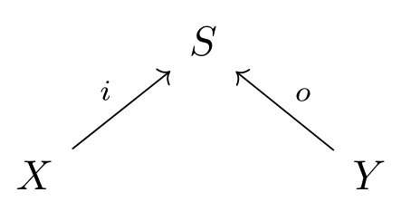
together with a vector field on . Here the legs of the cospan mark the species that we’re allowed to inject and remove, labeled () for input (output).
So, how can we build a category from this? Loosely citing a result of Fong, if the decorations of the cospan (in this case, the vector fields) can be given through a functor that is lax monoidal, then we can form a category whose objects are finite sets, and whose morphisms are (iso classes of) decorated cospans.
Indeed, this can be done in a very natural way, and therefore gives rise to the category , whose morphisms are open dynamical systems.
The black-boxing functor
Given a dynamical system, one of the first things we might like to do is to study its fixed points; in our case, study the concentration vectors that remain constant in time. When working with an open dynamical system, it’s clear that the amounts that we choose to inject and remove will alter the change in concentration of our species, and hence it makes sense to consider the following.
For an open dynamical system , together with a constant inflow and constant outflow , a steady state (with inflows and outflows ) is a constant vector of concentrations such that
Here is the vector in given by ; that is, the inflow concentration of all species as marked by the input leg of the cospan. As the authors concisely put it, “in a steady state, the inflows and outflows conspire to exactly compensate for the reaction velocities”.
Note that the inflow and outflow functions and won’t affect any species not marked by the legs of the cospan, and so any steady state must be such that when restricted to these inner species that we can’t reach.
What we want to do next is build a functor that, given an open dynamical system, records all possible combinations of input concentrations, output concentrations, inflows and outflows that hold in steady state. This process will be called black-boxing, since it discards information that can’t be seen at the inputs and outputs.
The black-boxing functor takes a finite set to the vector space , and a morphism, that is, an open dynamical system , to the subset
where is the vector in defined by ; that is, the concentration of the input species.
The authors prove that black-boxing is indeed a functor, which implies that if we want to study the steady states of a complex open dynamical system, we can break it up into smaller, simpler pieces and study their steady states. In other words, studying the steady states of a big system, which is given by the composition of smaller systems (as morphisms in the category ) amounts to studying the steady states of each of the smaller systems, and composing them (as morphisms in ).
Spivak’s approach
The category of wiring diagrams
Instead of dealing with dynamical systems from the start, Spivak takes a step back and develops a syntax for boxes, which are things that admit inputs and outputs.
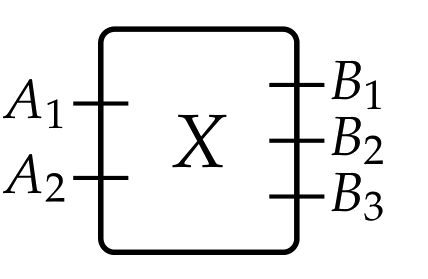
Let’s define the category of -boxes and wiring diagrams, for a category with finite products. Its objects are pairs
where each of these coordinates is a finite product of objects of . For example, we interpret the pair as a box with input ports and output ports .
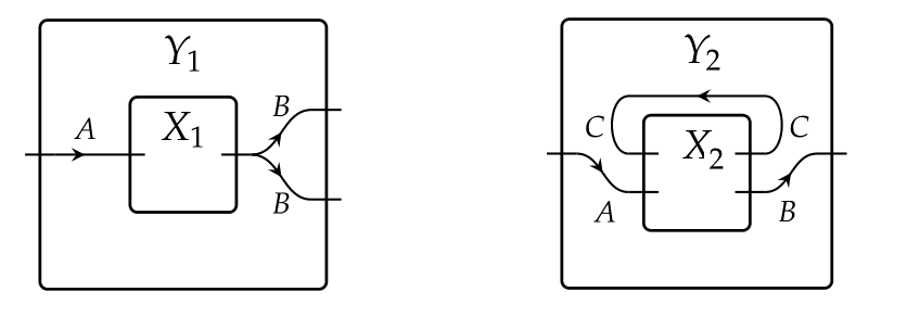
Its morphisms are wiring diagrams , that is, pairs of maps which we interpret as a rewiring of the box inside of the box . The function indicates whether an input port of should be attached to an input of or to an output of itself; the function indicates how the outputs of feed the outputs of . Examples of wirings are
Composition is given by a nesting of wirings.
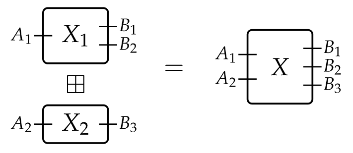
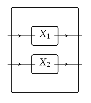
Given boxes and , we define their parallel composition by
This gives a monoidal structure to the category . Parallel composition is true to its name, as illustrated by
The huge advantage of this approach is that one can now fill the boxes with suitable “inhabitants”, and model many different situations that look like wirings at their core. These inhabitants will be given through functors , taking a box to the set of its desired interpretations, and giving a meaning to the wiring of boxes.
The functor of open dynamical systems
The first of our inhabitants will be, as you probably guessed by now, open dynamical systems. Here is the category of Euclidean spaces and smooth maps.
From the perspective of Spivak’s paper, an -open dynamical system is a 3-tuple where
is the state space
is a vector field parametrized by the inputs , giving the differential equation of the system
is the readout function at the outputs .
One should notice the similarity with our previously defined dynamical systems, although it’s clear that the two definitions are not equivalent.
The functor exhibiting dynamical systems as inhabitants of input-output boxes, takes a box to the set of all -dynamical systems
You can surely figure out how acts on wirings by drawing a picture and doing a bit of careful bookkeeping.
Note that there’s a natural notion of parallel composition of two dynamical systems, which amounts to carrying out the processes indicated by the two dynamical systems in parallel. Spivak shows that is a functor, and, furthermore, that
The functor of -matrices
Our second inhabitants will be given by matrices of sets. For objects , an -matrix of sets is a function that assigns to each pair a set . In other words, it is a matrix indexed by that, instead of coefficients, has sets in each position.
The functor exhibiting -matrices as inhabitants of input-output boxes, takes a box to the set of all -matrices of sets
Once again, it’s not too hard to figure out how should act on wirings.
Like before, there’s a notion of parallel composition of two matrices of sets, and the author shows that is a functor such that
The steady-state natural transformation
Finally, we explain how to use all this to study steady states of dynamical systems.
Given an -dynamical system and an element , an -steady state is a state such that
Since dynamical systems are encoded by the functor , it makes sense to study steady states through a natural transformation out of . We define as the transformation that assigns to each box , the function
taking a dynamical system to its matrix of steady states
where . The author proceeds to show that is a monoidal natural transformation.
Is it possible to use this machinery to draw the same conclusion as before, that is, that the steady states of a composition of systems comes from the composition of the steady states of the parts?
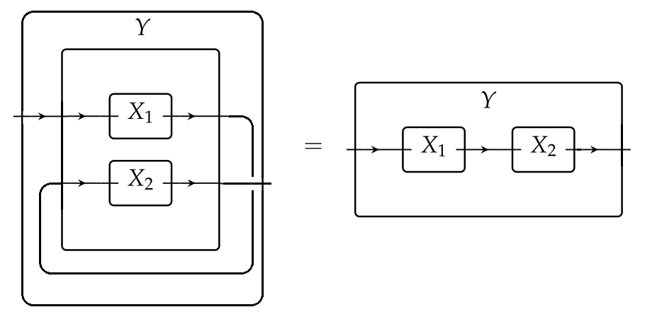
Indeed, it is! Given two boxes and , we recover the usual notion of (serial) composition by first setting them in parallel ,
and wiring this by as follows:
The fact that is a monoidal natural transformation, combined with the facts that the functors and respect parallel composition, allows us to write the following diagram, where both squares are commutative
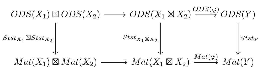
Then, chasing the diagram along the top and left sides gives the steady states of the serial composition of the dynamical systems and , while chasing it along the right and bottom sides gives the composition of the steady states of and of , and the two must agree.
The two approaches, side by side
So how are these two perspectives related? Looking at the definitions we can immediately see that Spivak’s approach has a broader scope than Baez and Pollard’s, so it’s apparent that his results won’t be implied by theirs.
For the converse direction, recall that in the first paper, a dynamical system is given by a decorated cospan , and a steady state with inflows and outflows is a constant vector of concentrations such that
Thus, studying the steady states for this cospan system corresponds to studying the box system
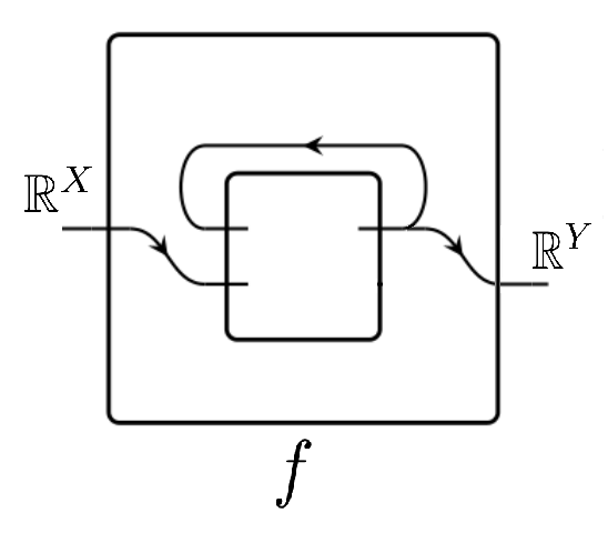
with dynamics given by , since its -steady states are vectors such that
Thus, the study of the steady states of a given cospan dynamical system can be done just as well by looking at it as a box dynamical system and running it through Spivak’s machinery. However, setting two such box systems in serial composition will not yield the box system representing the composition of the cospan systems as one would (naively?) hope, so it doesn’t seem that Spivak’s compositional results will imply those of Baez and Pollard.
This is a bit disconcerting, but instead of it being discouraging, I believe it should be seen as an invitation to delve into the semantics of open dynamical systems and find the right perspective, which manages to subsume both of the approaches presented here.
Re: Dynamical Systems and Their Steady States
Can Spivak’s formalism of open dynamical systems express the same sequential composition of dynamical systems as the Baez-Pollard Dynam?
Also this all smells very double categorical to me. I know Decorated Cospans come with a natural double category structure, maybe Spivak’s functors can be viewed that way too.