The Behavioral Approach to Systems Theory
Posted by John Baez
.")
guest post by Eliana Lorch and Joshua Tan
As part of the Applied Category Theory seminar, we discussed an article commonly cited as an inspiration by many papers1 taking a categorical approach to systems theory, The Behavioral Approach to Open and Interconnected Systems. In this sprawling monograph for the IEEE Control Systems Magazine, legendary control theorist Jan Willems poses and answers foundational questions like how to define the very concept of mathematical model, gives fully-worked examples of his approach to modeling from physical first principles, provides various arguments in favor of his framework versus others, and finally proves several theorems about the special case of linear time-invariant differential systems.
In this post, we’ll summarize the behavioral approach, Willems’ core definitions, and his “systematic procedure” for creating behavioral models; we’ll also examine the limitations of Willems’ framework, and conclude with a partial reference list of Willems-inspired categorical approaches to understanding systems.
The behavioral approach
Here’s the view from 10,000 feet of the behavioral approach in contrast with the traditional signal-flow approach:
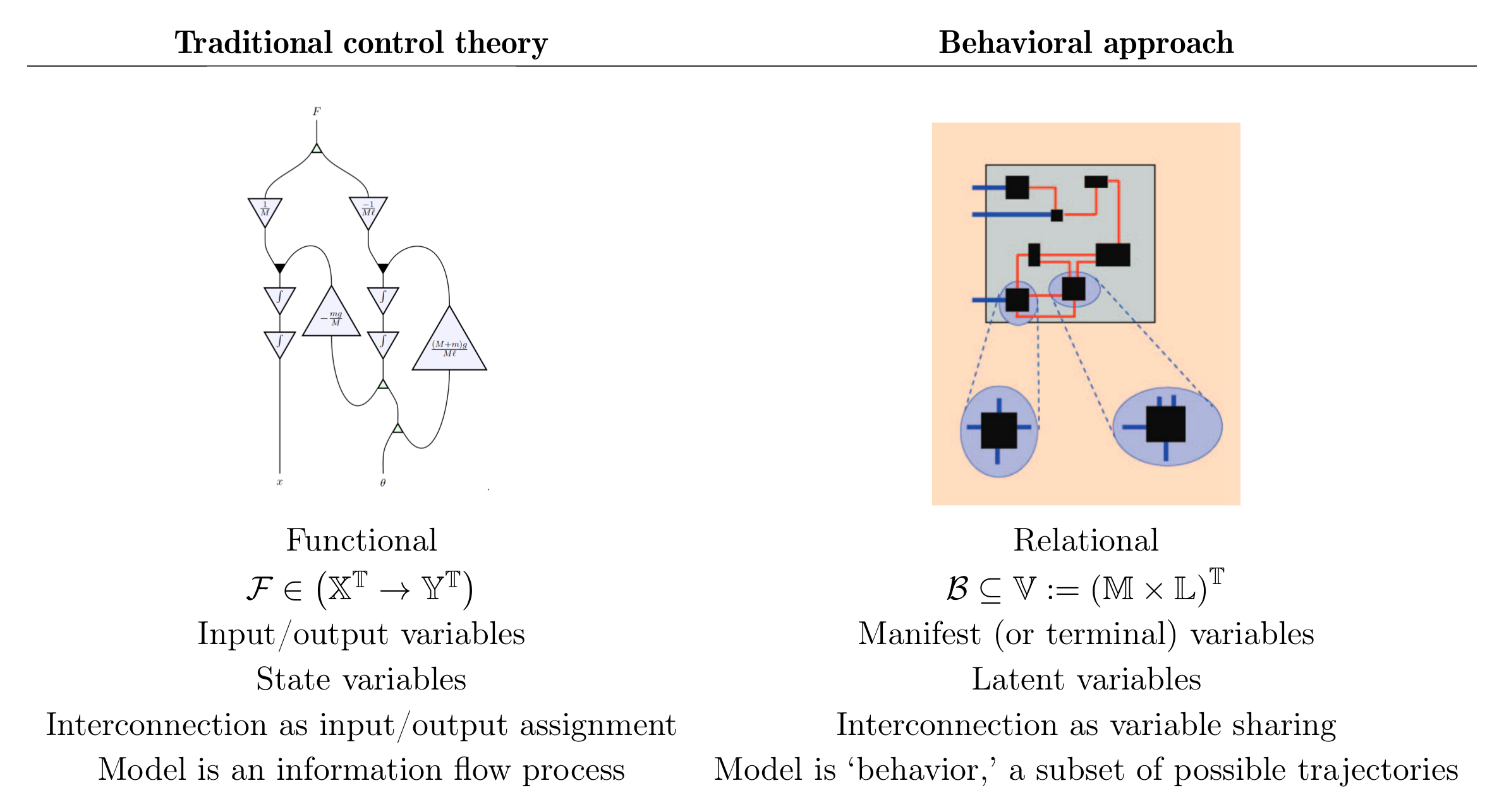
Willems’ approach breaks down into: (1) considering a dynamical system as a ‘behavior,’ and (2) defining interconnection as variable sharing.
Dynamical system as behavior
Willems goes so far as to claim: “It is remarkable that the idea of viewing a system in terms of inputs and outputs, in terms of cause and effect, kept its central place in systems and control theory throughout the 20th century. Input/output thinking is not an appropriate starting point in a field that has modeling of physical systems as one of its main concerns.”
To get a sense of the inappropriateness of input/output-based modeling: consider a freely swinging pendulum in 2-dimensional space with a finite-sized bob. Now consider adding to this system a model representing the right-hand half-plane being filled with cement. With soft-contact mechanics, we could determine what force the cement exerts on the pendulum when it bounces against it — that is, when the pendulum bob’s center of mass comes within its radius of the right half-plane.
Traditionally, we might define a function that takes the pendulum’s position as input and produces a force as output. But this is insufficient to model the effect of the wall, which also prevents the pendulum bob’s center of mass from ever being in the right-hand half-plane; the wall imposes a constraint on the possible states of the world. How can we can capture this kind of constraint? In this case, we can extend the state model with inequalities delineating the feasible region of the state space.2
Willems’ insight is that the entire modeling framework can be subsumed by a sufficiently broad notion of “feasible region.” A dynamical system is simply a relation on the variables, forming a subset of all conceivable trajectories — a ‘behavior.’
Interconnection as variable sharing
The signal-flow approach to systems modeling requires labeling the terminals of a system as inputs or outputs before a model can be formulated; Willems argues this does not respect the actual physics. Most physical terminals — electrical wires, mechanical linkages or gears, thermal couplings, etc. — do not have an intrinsic, a priori directionality, and may permit “signals” to “flow” in either or both directions. Rather, physical interconnections constrain certain variables on either side to be equal (or equal-and-opposite). After having modeled a system, one may be able to prove that it obeys a certain partitioning of variables into inputs and outputs, but assuming this up front obscures the underlying physical reality. This paradigm shift amounts to moving from functional composition (given we compute , then ) to relational composition: iff , which can be read as “variable sharing” between and . This is a way of restoring symmetry to composition — giving no precedence either between the two entities being composed, nor between each entity’s domain and codomain.
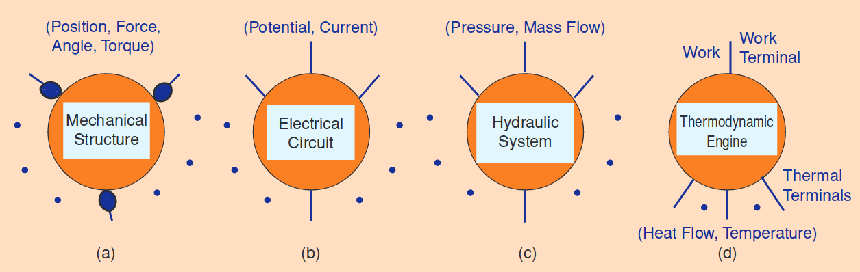
Examples of systems to model within the behavioral framework.
Core definitions
Given some natural phenomenon we wish to model mathematically, the first step is to establish the universum, the set of all a priori feasible outcomes, notated . Then, Willems asserts a mathematical model to be a restriction of possible outcomes to a subset of .3 This subset itself is called the behavior of the model, and is written . This concept is, as the name suggests, at the center of Willems’ “behavioral approach”: he asserts that “equivalence of models, properties of models, model representations, and system identification must refer to the behavior.”
A dynamical system is a model in which elements of the universum are functions of time, that is, a triple
in which . is referred to as the time set (which may be discrete or continuous), and is referred to as the signal space. The elements of are trajectories .
A dynamical system with latent variables is one whose signal space is a Cartesian product of manifest variables and latent variables: the “full” system is a tuple
where the behavior . Here is the set of manifest values and is the set of latent values.
A full behavior is said to induce or represent a manifest dynamical system , with the manifest behavior defined by
The behavior of all the variables is determined by the equations specifying the first-principles physical laws, together with the equations expressing all the constraints from interconnection. Willems treats interconnection as simply “variable sharing,” that is, restricting behavior such that the trajectories assigned to the interconnected variables are constrained to be equal (or sometimes “equal and opposite,” depending on sign conventions).
An interconnection architecture is a sort of wiring diagram (analogous to operadic wiring diagrams) that describes the way in which a collection of systems is interconnected. Willems formalises this as a graph with leaves: a set of vertices (which are systems or modules), a set of edges (terminals), and a set of leaves (open wires), with an assignment map : to each edge an unordered pair of vertices and to each leaf a single vertex. A leaf is depicted as an open half-edge emanating from the graph, like a wire sticking out of a circuit — the “open” part of “open and interconnected systems.” (Note that this interpretation of a “leaf” differs from the usual graph-theoretic “vertex with degree one”; here, a leaf is like an “edge with degree one.”) There’s a type-checking condition that the set of leaves and internal half-edges emanating from a vertex must be completely matched to the set of terminals of the associated module, so that you don’t have hidden dangling wires.
Finally, the interconnection architecture requires a module embedding that specifies how each vertex is interpreted as a module: either a primitive model made of physical laws, or a sub-model within which there’s a further module embedding. Here we get a sense of the “zooming” nature of the modeling procedure.
Tearing, Zooming, Linking
Willems proposes a “systematic procedure” for generating models in this behavioral form: first decompose (tear) the system under investigation into smaller subsystems, then recursively apply the modeling process (zoom in) to each subsystem, and finally compose (link) the resulting submodels together into an overall system model. Rendered in pseudocode, it looks like this:
define makeModel(System system) => Model {
  if (system is directly governed by known physics) {
    return knownModel(system)
  } else {
    WiringDiagram<System> decomposition := tear(system)
    List<Model> submodels := decomposition.listSubsystems().fmap(makeModel)
    return decomposition.link(submodels)
  }
}
As an example, Willems analyzes an open hydraulic system made of two tanks interconnected by a pipe:
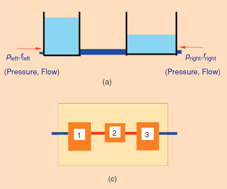
In the “tear” step, he breaks the system apart into three subsystems: the two tanks, (1) and (3) in the figure, and the pipe (2). In the “zoom” step, each of the three subsystems is “simple enough to be modeled using first-principles physical laws,” so he fills in the known model for each one (reaching the recursive base case, rather than starting again from “tear”). For the pipe, flows on each end are equal and opposite, and the difference in pressure is proportional to the flow; for each of the tanks, conservation of mass and Bernoulli’s laws relate the pressures, flows, and height of water in the tank.
Then, in the “link” step, he starts with, for each subsystem, a copy of the corresponding model (initially each relating a completely separate set of variables), then combines the models according to the links between subsystems, using the appropriate “interconnection laws” for each pair of connected terminals. In this example, the interconnection laws consist of setting connected pressures to be equal and connected flows to be equal and opposite.
An essential claim of Willems’ philosophy is that for physical systems for which we can use his modeling procedure of breaking systems into subsystems with interconnections, the hierarchical structure of our model will match reality closely enough that there will be straightforward physical principles governing the interactions at the interfaces (which tend to correspond to partitions of physical space). Many engineered systems deliberately have their important interfaces clearly delineated, but he explicitly disclaims that there are forms of interaction, such as gravitational interaction and colliding objects, which do not perfectly fit this framework.
Limitations of Willems’ framework
Not all interconnections fit. This framework assumes that the interface of a module can be specified—as a finite set of terminals—prior to composition with other modules, and Willems identifies three situations where this assumption fails:
-body problems exhibiting “virtual terminals” which are not so much a property of each module, but of each pair of modules. The classic example of this phenomenon is the -body problem in gravitational (or electrostatic, etc.) dynamics: an -body system has interactions, but the combination of an -body system and an -body system has more than interactions.
“Distributed interconnections” in which a terminal has continuous spatial extent (e.g. heat conduction along a surface), calling for partial differential equations involving coordinate variables.
Contact mechanics such as rolling, sliding, bouncing, collisions, etc., in which interconnections appear and vanish depending on the values of certain position variables, as objects come into and out of contact.
Directional components and systems. In contrast to an a posteriori partitioning of variables into inputs and outputs (meaning that any setting of the “inputs” uniquely determines the trajectories of the “outputs”), some components fundamentally exhibit a priori input/output behavior (that is, they cannot be back-driven), and Willems’ framework can’t accommodate these.
Ideal amplifier. The behavior of an ideal amplifier with gain , input and output would be (constant-gain model), yet Willems’ approach here would make the incorrect prediction that we could back-drive terminal by interconnecting it to a signal source and expect to observe the signal scaled by at terminal . However, an “ideal amplifier” is not a first-principles physical law; the modeling procedure might suggest we “tear” an amplifier further into its component parts, and then “tear” the constituent transistors with a deconstruction (such as the Gummel-Poon model) into passive circuit primitives. This might result in a more realistic model of actual amplifier behavior, though it would have at least an order of magnitude more components than the constant-gain model.
Humans, etc. Willems lists additional signal-flow systems for which the behavioral approach is not quite adequate: actuator inputs and sensor outputs interconnected via a controller, reactions of humans or animals, devices that respond to external commands, or switches and other logical devices.
Cartesian latent/manifest partitioning. Among Willems’ arguments against mandatory input/output partitioning is the simple and compelling example of a particle moving on a sphere, whose position is truly an output and whose velocity is truly an input—yet even in this seemingly favorable setup, the full state space (the tangent bundle of the sphere) cannot be decomposed as a Cartesian product of positions on the sphere with any vector space. However, Willems uses exactly the same hidden assumption in his definition of a dynamical system with latent variables. If a dynamical system’s full state space can’t be written as a Cartesian product, then its behavior can’t be represented in the way Willems defines.
Probability. Willems’ non-deterministic approach to behaviors is a kind of unquantified uncertainty; it doesn’t natively give us a way of associating probabilities with elements of a “behavior” (although behaviors could be considered as always having an implicitly uniform distribution). Nontrivial distributions could also be modeled by defining the universum (where is probability, namely the Giry monad), but the non-determinism of introduces “Knightian uncertainty”, in that models are now sets of distributions, with no probabilities specified at the top level—and it’s unclear how such models should compose with non-stochastic models.
Categorical approaches to systems
As mentioned earlier, Willems has been an inspiration for many papers in applied category theory. One common feature is that many take a relational approach to semantics, providing a functor into (some subcategory of) . Here is a (non-exhaustive!) reference list of these and related works.
Applications to specific domains:
Passive linear networks: Baez and Fong, 2015. Constructs a “black-boxing” functor from a decorated-cospan category of passive linear circuits (composed of resistors, inductors and capacitors) to a behavior category of Lagrangian relations.
Generalized circuit networks: Baez, Coya and Rebro, 2018. Generalizes the black-boxing functor to potentially nonlinear components/circuits.
Reversible Markov processes: Baez, Fong and Pollard, 2016. Constructs a “black-boxing” functor from a decorated-cospan category of reversible Markov processes to a category of linear relations describing steady states.
Petri nets / reaction networks: Baez and Pollard, 2017. Constructs a “black-boxing” functor from a decorated-cospan category of Petri nets to a category of semi-algebraic relations describing steady states, with an intermediate stop at a “grey-box” category of algebraic vector fields.
Digital circuits: Ghica, Jung and Lopez, 2017. Defines a symmetric monoidal theory of circuits including a discrete-delay operator and feedback, with operational semantics.
Discrete linear time-invariant dynamical systems (LTIDS): Fong, Sobocinski, and Rapisarda, 2016. Constructs a full and faithful functor from a freely generated symmetric monoidal theory into the PROP of LTIDSs and characterizes controllability in terms of spans, among other things—not only using Willems’ definitions and philosophy, but even some of his theorems.
General frameworks:
Algebra of Open and Interconnected Systems: Brendan Fong’s 2016 doctoral thesis. Covers his technique of decorated cospans as well as more recent work on decorated corelations, both of which are especially useful to construct syntactic categories for various kinds of non-categorical diagrams.
Topos of behavior types: Schultz and Spivak, 2017. Constructs a temporal type theory, as the internal logic of the category of sheaves on an interval domain, in which every object represents a behavior that seems to be essentially in Willems’ sense of the word.
Operad of wiring diagrams: Vagner, Spivak and Lerman, 2015. Formalises construction of systems of differential equations on manifolds using Spivak’s “operad of wiring diagrams” approach to composition, which is conceptually similar to Willems’ notion of hierarchical zooming into modules.
Signal flow graphs: Bonchi, Sobocinski and Zanasi, 2017. Sound and complete axiomatization of signal flow graphs, arguably the primary incumbent against which Willems’ behavioral approach contends.
Bond graphs: Brandon Coya, 2017. Defines a category of bond graphs (an older general modeling framework which Willems acknowledges as a step in the right direction toward a behavioral approach) with functorial semantics as Lagrangian relations.
Cospan/Span(Graph): Gianola, Kasangian and Sabadini in 2017 review a line of work mostly done in the 90’s by Sabadini, Walters and collaborators on what are essentially open and interconnected labeled-transition systems.
Many thanks to Pawel Sobocinski and Brendan Fong for feedback on this post, and to Sophie Raynor and other members of the seminar for thoughts and discussions.
1 see e.g. Spivak and Schultz’s Temporal type theory; Fong, Sobocinski, and Rapisarda’s Categorical approach to open and interconnected dynamical systems; Bonchi, Sobocinski, and Zanasi’s Categorical semantics of signal flow graphs
2 Depending on the formalisation, a system of differential equations could technically contain equality constraints without any actual derivatives, such as , which can restrict the feasible region without augmenting the modeling framework to include inequalities. We could even impose the constraint by using a non-analytic function:
3 Note: From a computer science perspective, this says that any “mathematical model” must be a non-deterministic model, as opposed to, on the one hand, a deterministic model (which would pick out an element of ), or, on the other hand, a probabilistic model (which would give a distribution over ). If we are given free choice of , any of these kinds of model is encodable as any other, but the choice is significant when it comes to composition.
Re: The Behavioral Approach to Systems Theory
Re: -body problems, the fast multipole method can be thought of as a way to reduce interactions to in the way needed to make Willems’ perspective work. More generally, renormalization group ideology is essentially that in cases where decomposition can be meaningful in light of the RG, one ought still to be able to justify Willems’ perspective along the lines I sketched at NIST in March.