Circuits, Bond Graphs, and Signal-Flow Diagrams
Posted by John Baez
.")

My student Brandon Coya finished his thesis, and successfully defended it last Tuesday!
• Brandon Coya, Circuits, Bond Graphs, and Signal-Flow Diagrams: A Categorical Perspective, Ph.D. thesis, U. C. Riverside, 2018.
It’s about networks in engineering. He uses category theory to study the diagrams engineers like to draw, and functors to understand how these diagrams are interpreted.
His thesis raises some really interesting pure mathematical questions about the category of corelations and a ‘weak bimonoid’ that can be found in this category. Weak bimonoids were invented by Pastro and Street in their study of ‘quantum categories’, a generalization of quantum groups. So, it’s fascinating to see a weak bimonoid that plays an important role in electrical engineering!
However, in what follows I’ll stick to less fancy stuff: I’ll just explain the basic idea of Brandon’s thesis, say a bit about circuits and ‘bond graphs’, and outline his main results. What follows is heavily based on the introduction of his thesis, but I’ve baezified it a little.
The basic idea
People, and especially scientists and engineers, are naturally inclined to draw diagrams and pictures when they want to better understand a problem. One example is when Feynman introduced his famous diagrams in 1949; particle physicists have been using them ever since. But some other diagrams introduced by engineers are far more important to the functioning of the modern world and its technology. It’s outrageous, but sociologically understandable, that mathematicians have figured out more about Feynman diagrams than these other kinds: circuit diagrams, bond graphs and signal-flow diagrams. This is the problem Brandon aims to fix.
I’ve been unable to track down the early history of circuit diagrams, so if you know about that please tell me! But in the 1940s, Harry Olson pointed out analogies in electrical, mechanical, thermodynamic, hydraulic, and chemical systems, which allowed circuit diagrams to be applied to a wide variety of fields. And on April 24, 1959, Henry Paynter woke up and invented the diagrammatic language of bond graphs to study generalized versions of voltage and current, called ‘effort’ and ‘flow,’ which are implicit in the analogies found by Olson. Bond graphs are now widely used in engineering. On the other hand, control theorists use diagrams of a different kind, called ‘signal-flow diagrams’, to study linear open dynamical systems.
Although category theory predates some of these diagrams, it was not until the 1980s that Joyal and Street showed string digrams can be used to reason about morphisms in any symmetric monoidal category. This motivates Brandon’s first goal: viewing electrical circuits, signal-flow diagrams, and bond graphs as string diagrams for morphisms in symmetric monoidal categories.
This lets us study networks from a compositional perspective. That is, we can study a big network by describing how it is composed of smaller pieces. Treating networks as morphisms in a symmetric monoidal category lets us build larger ones from smaller ones by composing and tensoring them: this makes the compositional perspective into precise mathematics. To study a network in this way we must first define a notion of ‘input’ and ‘output’ for the network diagram. Then gluing diagrams together, so long as the outputs of one match the inputs of the other, defines the composition for a category.
Network diagrams are typically assigned data, such as the potential and current associated to a wire in an electrical circuit. Since the relation between the data tells us how a network behaves, we call this relation the ‘behavior’ of a network. The way in which we assign behavior to a network comes from first treating a network as a ‘black box’, which is a system with inputs and outputs whose internal mechanisms are unknown or ignored. A simple example is the lock on a doorknob: one can insert a key and try to turn it; it either opens the door or not, and it fulfills this function without us needing to know its inner workings. We can treat a system as a black box through the process called ‘black-boxing’, which forgets its inner workings and records only the relation it imposes between its inputs and outputs.
Since systems with inputs and outputs can be seen as morphisms in a category we expect black-boxing to be a functor out of a category of this sort. Assigning each diagram its behavior in a functorial way is formalized by functorial semantics, first introduced in Lawvere’s thesis in 1963. This consists of using categories with specific extra structure as ‘theories’ whose ‘models’ are structure-preserving functors into other such categories. We then think of the diagrams as a syntax, while the behaviors are the semantics. Thus black-boxing is actually an example of functorial semantics. This leads us to another goal: to study the functorial semantics, i.e. black-boxing functors, for electrical circuits, signal-flow diagrams, and bond graphs.
Brendan Fong and I began this type of work by showing how to describe circuits made of wires, resistors, capacitors, and inductors as morphisms in a category using ‘decorated cospans’. Jason Erbele and I, and separately Bonchi, Sobociński and Zanasi, studied signal flow diagrams as morphisms in a category. In other work Brendan Fong, Blake Pollard and I looked at Markov processes, while Blake and I studied chemical reaction networks using decorated cospans. In all of these cases, we also studied the functorial semantics of these diagram languages.
Brandon’s main tool is the framework of ‘props’, also called ‘PROPs’, introduced by Mac Lane in 1965. The acronym stands for “products and permutations”, and these operations roughly describe what a prop can do. More precisely, a prop is a strict symmetric monoidal category equipped with a distinguished object such that every object is a tensor power Props arise because very often we think of a network as going between some set of input nodes and some set of output nodes, where the nodes are indistinguishable from each other. Thus we typically think of a network as simply having some natural number as an input and some natural number as an output, so that the network is actually a morphism in a prop.
Circuits and bond graphs
Now let’s take a quick tour of circuits and bond graphs. Much more detail can be found in Brandon’s thesis, but this may help you know what to picture when you hear terminology from electrical engineering.
Here is an electrical circuit made of only perfectly conductive wires:
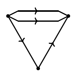
This is just a graph, consisting of a set of nodes, a set of edges, and maps sending each edge to its source and target node. We refer to the edges as perfectly conductive wires and say that wires go between nodes. Then associated to each perfectly conductive wire in an electrical circuit is a pair of real numbers called ‘potential’, and ‘current’,

Typically each node gets a potential, but in the above case the potential at either end of a wire would be the same so we may as well associate the potential to the wire. Current and potential in circuits like these obey two laws due to Kirchoff. First, at any node, the sum of currents flowing into that node is equal to the sum of currents flowing out of that node. The other law states that any connected wires must have the same potential.
We say that the above circuit is closed as opposed to being open because it does not have any inputs or outputs. In order to talk about open circuits and thereby bring the ‘compositional perspective’ into play we need a notion for inputs and outputs of a circuit. We do this using two maps and that specifiy the inputs and outputs of a circuit. Here is an example:
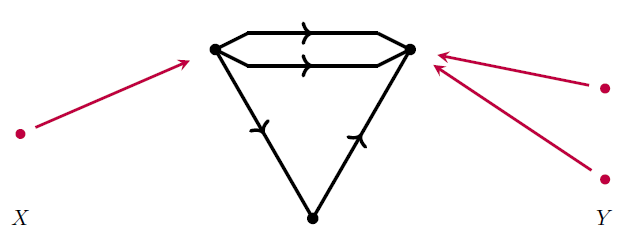
We call the sets and the disjoint union the inputs, outputs, and terminals of the circuit, respectively. To each terminal we associate a potential and current. In total this gives a space of allowed potentials and currents on the terminals and we call this space the ‘behavior’ of the circuit. Since we do this association without knowing the potentials and currents inside the rest of the circuit we call this process ‘black-boxing’ the circuit. This process hides the internal workings of the circuit and just tells us the relation between inputs and outputs. In fact this association is functorial, but to understand the functoriality first requires that we say how to compose these kinds of circuits. We save this for later.
There are also electrical circuits that have ‘components’ such as resistors, inductors, voltage sources, and current sources. These are graphs as above, but with edges now labelled by elements in some set L. Here is one for example:
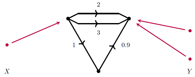
We call this an L-circuit. We may also black-box an L-circuit to get a space of allowed potentials and currents, i.e. the behavior of the L-circuit, and this process is functorial as well. The components in a circuit determine the possible potential and current pairs because they impose additional relationships. For example, a resistor between two nodes has a resistance and is drawn as:
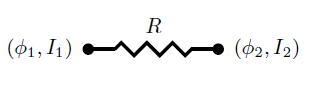
In an L-circuit this would be an edge labelled by some positive real number For a resistor like this Kirchhoff’s current law says and Ohm’s Law says This tells us how to construct the black-boxing functor that extracts the right behavior.
Engineers often work with wires that come in pairs where the current on one wire is the negative of the current on the other wire. In such a case engineers care about the difference in potential more than each individual potential. For such pairs of perfectly conductive wires:
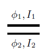
we call the ‘voltage’ and the ‘current’. Note the word current is used for two different, yet related concepts. We call a pair of wires like this a ‘bond’ and a pair of nodes like this a ‘port’. To summarize we say that bonds go between ports, and in a ‘bond graph’ we draw a bond as follows:

Note that engineers do not explicitly draw ports at the ends of bonds; we follow this notation and simply draw a bond as a thickened edge. Engineers who work with bond graphs often use the terms ‘effort’ and ‘flow’ instead of voltage and current. Thus a bond between two ports in a bond graph is drawn equipped with an effort and flow, rather than a voltage and current, as follows:

A bond graph consists of bonds connected together using ‘1-junctions’ and ‘0-junctions’. These two types of junctions impose equations between the efforts and flows on the attached bonds. The flows on bonds connected together with a 1-junction are all equal, while the efforts sum to zero, after sprinkling in some signs depending on how we orient the bonds. For 0-junctions it works the other way: the flows are all equal while the efforts sum to zero! The duality here is well-known to engineers but perhaps less so to mathematicians. This is one topic Brandon’s thesis explores.
Brandon explains bond graphs in more detail in Chapter 5 of his thesis, but here is an example:
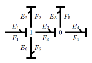
The arrow at the end of a bond indicates which direction of current flow counts as positive, while the bar is called the ‘causal stroke’. These are unnecessary for Brandon’s work, so he adopts a simplified notation without the arrow or bar. In engineering it’s also important to attach general circuit components, but Brandon doesn’t consider these.
Outline
In Chapter 2 of his thesis, Brandon provides the necessary background for studying four categories as props:
• the category of finite sets and spans:
• the category of finite sets and relations:
• the category of finite sets and cospans:
• the category of finite sets and corelations: .
In particular, and are crucial to the study of networks.
In Corollary 2.3.4 he notes that any prop has a presentation in terms of generators and equations. Then he recalls the known presentations for and . Proposition 2.3.7 lets us build props as quotients of other props.
He begins Chapter 3 by showing that is ‘the prop for extraspecial commutative Frobenius monoids’, based on a paper he wrote with Brendan Fong. This result also gives a presentation for
Then he defines an “L-circuit” as a graph with specified inputs and outputs where all the edge are labeled by elements of some set L. L-circuits are morphisms in the prop In Proposition 3.2.8 he uses a result of Rosebrugh, Sabadini and Walters to show that can be viewed as the coproduct of and the free prop on the set L of labels.
Brandon then defines to be the prop where L consists of a single element. This example is important, because can be seen as the category whose morphisms are circuits made of only perfectly conductive wires! From any morphism in he extracts a cospan of finite sets and then turns the cospan into a corelation. These two processes are functorial, so he gets a method for sending a circuit made of only perfectly conductive wires to a corelation:
There is also a functor
where is the category whose objects are finite dimensional vector spaces and whose morphisms are linear relations, that is, linear subspaces By composing with the above functors and he associates a linear relation to any circuit made of perfectly conductive wires. On the other hand he gets a subspace for any such circuit by first assigning potential and current to each terminal, and then subjecting these variables to the appropriate physical laws.
It turns out that these two ways of assigning a subspace to a morphism in are the same. So, he calls the linear relation associated to a circuit using the composite the “behavior” of the circuit and defines the “black-boxing” functor
to be this composite.
Note that the underlying corelation of a circuit made of perfectly conductive wires completely determines the behavior of the circuit via the functor
In Chapter 4 he reinterprets the black-boxing functor as a morphism of props. He does this by introducing the category whose objects are “symplectic” vector spaces and whose morphisms are “Lagrangian” relations. In Proposition 4.1.6 he proves that the functor actually picks out a Lagrangian relation for any corelation and thus determines a morphism of props. So, he redefines to be this morphism
and reinterprets black-boxing as the composite
After doing all this hard work for circuits made of perfectly conductive wires — a warmup exercise that engineers might scoff at — Brandon shows the power of his results by easily extending the black-boxing functor to circuits with arbitrary label sets in Theorem 4.2.1. He applies this result to a prop whose morphisms are circuits made of resistors, inductors, and capacitors. Then he considers a more general and mathematically more natural approach to linear circuits using the prop The morphisms here are open circuits with wires labelled by elements of some chosen field In Theorem 4.2.4 he prove the existence of a morphism of props
that describes the black-boxing of circuits built from arbitrary linear components.
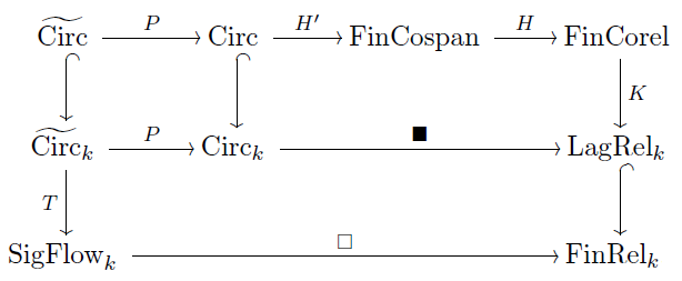
Brandon then picks up where Jason Erbele’s thesis left off, and recalls how control theorists use “signal-flow diagrams” to draw linear relations. These diagrams make up the category , which is the free prop generated by the same generators as . Similarly he defines the prop as the free prop generated by the same generators as . Then there is a strict symmetric monoidal functor giving a commutative square:
Of course, circuits made of perfectly conductive wires are a special case of linear circuits. We can express this fact using another commutative square:
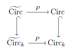
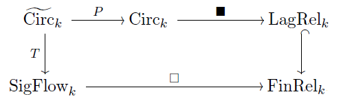
Combining the diagrams so far, Brandon gets a commutative diagram summarizing the relationship between linear circuits, cospans, corelations, and signal-flow diagrams:
Brandon concludes Chapter 4 by extending his work to circuits with voltage and current sources. These types of circuits define affine relations instead of linear relations. The prop framework lets Brandon extend black-boxing to these types of circuits by showing that affine Lagrangian relations are morphisms in a prop This leads to Theorem 4.4.5, which says that for any field and label set L there is a unique morphism of props
extending the other black-boxing functor and sending each element of L to an arbitrarily chosen affine Lagrangian relation between potentials and currents.
In Chapter 5, Brandon study bonies graphs as morphisms in a category. His goal is to define a category whose morphisms are bond graphs, and then assign a space of efforts and flows as behavior to any bond graph using a functor. He also constructs a functor that assigns a space of potentials and currents to any bond graph, which agrees with the way that potential and current relate to effort and flow.
The subtle way he defines comes from two different approaches to studying bond graphs, and the problems inherent in each approach. The first approach leads him to a subcategory of , while the second leads him to a subcategory of . There isn’t a commutative square relating these four categories, but Brandon obtains a pentagon that commutes up to a natural transformation by inventing a new category :
This category is a way of formalizing Paynter’s idea of bond graphs.
In his first approach, Brandon views a bond graph as an electrical circuit. He takes advantage of his earlier work on circuits and corelations by taking to be the category whose morphisms are circuits made of perfectly conductive wires. In this approach a terminal is the object 1 and a wire is the identity corelation from 1 to 1, while a circuit from m terminals to n terminals is a corelation from m to n.
In this approach Brandon thinks of a port as the object 2, since a port is a pair of nodes. Then he thinks of a bond as a pair of wires and hence the identity corelation from 2 to 2. Lastly, the two junctions are two different ways of connecting ports together, and thus specific corelations from 2m to 2n. It turns out that by following these ideas he can equip the object 2 with two different Frobenius monoid structures, which behave very much like 1-junctions and 0-junctions in bond graphs!
It would be great if the morphisms built from these two Frobenius monoids corresponded perfectly to bond graphs. Unfortunately there are some equations which hold between morphisms made from these Frobenius monoids that do not hold for corresponding bond graphs. So, Brandon defines a category using the morphisms that come from these two Frobenius monoids and moves on to a second attempt at defining .
Since bond graphs impose Lagrangian relations between effort and flow, this second approach starts by looking back at . The relations associated to a 1-junction make into yet another Frobenius monoid, while the relations associated to a 0-junction make into a different Frobenius monoid. These two Frobenius monoid structures interact to form a bimonoid! Unfortunately, a bimonoid has some equations between morphisms that do not correspond to equations between bond graphs, so this approach also does not result in morphisms that are bond graphs. Nonetheless, Brandon defines a category using the two Frobenius monoid structures
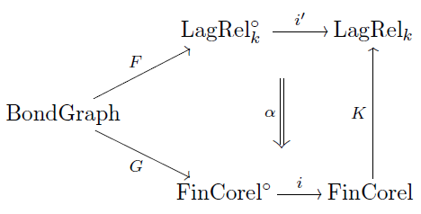
Since it turns out that and have corresponding generators, Brandon defines as a prop that also has corresponding generators, but with only the equations found in both and By defining in this way he automatically gets two functors
and
The functor associates effort and flow to a bond graph, while the functor lets us associate potential and current to a bond graph using the previous work done on Then the Lagrangian subspace relating effort, flow, potential, and current:
defines a natural transformation in the following diagram:
Putting this together with the diagram we saw before, Brandon gets a giant diagram which encompasses the relationships between circuits, signal-flow diagrams, bond graphs, and their behaviors in category theoretic terms:
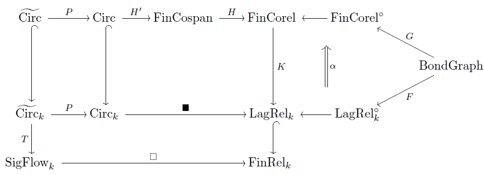
This diagram is a nice quick road map of his thesis. Of course, you need to understand all the categories in this diagram, all the functors, and also their applications to engineering, to fully appreciate what he has accomplished! But his thesis explains that.
To learn more
Coya’s thesis has lots of references, but if you want to see diagrams at work in actual engineering, here are some good textbooks on bond graphs:
• D. C. Karnopp, D. L. Margolis and R. C. Rosenberg, System Dynamics: A Unified Approach, Wiley, New York, 1990.
• F. T. Brown, Engineering System Dynamics: A Unified Graph-Centered Approach, Taylor and Francis, New York, 2007.
and here’s a good one on signal-flow diagrams:
• B. Friedland, Control System Design: An Introduction to State-Space Methods, S. W. Director (ed.), McGraw–Hill Higher Education, 1985.


Re: Circuits, Bond Graphs, and Signal-Flow Diagrams
small typo: “For 0-junctions it works the other way: the efforts are all equal while the efforts sum to zero!”