The n-Category Café

A quick introduction to monads

If you are already familiar with monads, you may skip this section. For everybody else, a monad on a category $C$ is one of the most important constructions in category theory. It consists of the following (subject to axioms you can find at the above link):

• an endofunctor $T\colon C\to C$ on our category;
• a natural transformation $\mu\colon T T\to T$, called the multiplication of the monad;
• a natural transformation $\eta\colon 1\to T$ from the identity on $C$ to $T$, called the unit of the monad.

A way to interpret and motivate the construction is the idea that a monad is like a consistent way of extending spaces to include generalized elements of a specific kind.

• The endofunctor $T\colon C\to C$ takes a space $X$ and gives a new space $T X$ which can be thought of as an extension of $X$.
• The unit natural transformation $\eta\colon 1\to T$ gives embeddings $X\to T X$ from the old spaces $X$ into their extensions $T X$. In other words, the new extended spaces have to contain the old ones.
• The multiplication natural transformation $\mu\colon T T\to T$ takes a extended extended space (twice) and maps it back to a one-time extended space.

As an example, take the power set monad on the category of sets.

• The endofunctor $T$ takes a set $X$ and gives the set $T X$ of its subsets. Subsets can be considered a generalization of elements.
• The unit gives maps $X\to T X$ which assign to $x\in X$ the singleton $\{x\}\in T X$. In this sense a subset is more general than an element: the elements correspond precisely to the subsets which are singletons.
• The multiplication $\mu\colon T T\to T$ maps subsets of subsets of $X$ into their union, which is a subset of $X$. For example,

$$\{\{x,y\}, \{x,z\}\} \;\mapsto\; \{x,y,z\} .$$

Another motivation for the theory monads is that a monad is like a consistent choice of spaces of formal expressions of a specific kind. In this interpretation, the endofunctor $T\colon C\to C$ takes a space $X$ and gives a new space $T X$ which can be thought of as containing formal expressions of a specific kind. One example is that of formal sums. If $X$ contains elements

$$x,y,z,\dots$$

then $T X$ contains finite strings such as

$$x + y + z, \; x + x, \; z.$$

The unit gives maps $X\to T X$ which assign to each element of $x$ the trivial formal expression containing only that one element. For example, for the formal sum case, $x$ is mapped to the trivial formal sum

$$x$$

in which nothing else is added to $x$.

The multiplication gives maps from formal sums of formal sums (twice) to formal sums, which reduce the expression by removing the nesting. For example,

$$(x + y) + (z + t) \; \mapsto \; x + y + z + t .$$

So far, all the operations are purely formal. There are spaces where these expressions can actually evaluated. For example, the sum

$$3+4+5$$

has the result $9$. The spaces where these formal expressions have a result are called the algebras of the monad. In particular, an algebra of the monad $T$ consists of an object $A$ together with a map $T A\to A$ which intuitively assigns to an expression its result. Again, the map is required to satisfy some axioms (which say, for example, that the trivial formal expression $x$ has result $x$).

For a more detailed but still nontechnical introduction to monads you can take a look at Chapter 1 of my thesis (pdf).

Probability monads

The idea of a probability monad is that we want to assign to a space $X$ a new space $P X$ containing random elements of $X$. This is consistent with the two interpretations given above:

• random elements can be thought of as a generalization of ordinary elements;
• random elements can be thought of as formal convex combinations of ordinary elements.

Probability monads were introduced by Michèle Giry in her work A Categorical approach to probability theory (pdf). A possible way of interpreting her work is the following. First of all we consider a “base” category $C$, whose objects we think of as spaces of possible outcomes, and whose morphisms we think of as functions between such spaces. For example, the outcomes of a coin flip form a set of two elements, $\{Heads, Tails\}$. Spaces of outcomes may have additional structure, usually at least a sigma-algebra, or even a topology or metric, and the morphisms of $C$ are compatible with that extra structure.

The category $C$ is equipped with a monad $(P, E, \delta)$, called probability monad, consisting of an endofunctor $P$, and natural transformations $E\colon P P\to P$ and $\delta\colon 1\to P$. Let’s see more in detail what these encode.

To each space of outcomes $X$, the functor $P$ assigns a space $P X$ of random outcomes. Usually, these are the probability measures on $X$,or sometimes valuations. For example, $P \{Heads, Tails\}$ contains all formal convex combinations, that is formal real linear combinations with the coefficients lying between $0$ and $1$ and adding to $1$. Here are some examples:

• $0 \,Heads + 1\, Tails$,
• $\frac{1}{2}\, Heads + \frac{1}{2}\, Tails$,
• $1\, Heads + 0\, Tails$,
• $\frac{3}{4}\, Heads + \frac{1}{4}\, Tails$.

For each space $X$, the unit $\delta$ gives a natural map from $X$ into the space $P X$ of random elements. It is usually an embedding, and it maps each (deterministic) outcome $x\in X$ to the outcome assigning probability $1$ to $x$ and $0$ to everything else. The outcomes in the image of $\delta$ are, in other words, those that are not really random. For the example of the coin, we have

• $\delta(Heads) = 1\, Heads + 0\, Tails$
• $\delta(Tails) = 0\, Heads + 1\, Tails$.

For each space $X$, the multiplication gives a natural map $P P X \to P X$. The space $P P X$ can be thought of as containing laws of random variables whose law is also random, or “random random variables”.

Here is an example. Suppose that I have two different coins in my pocket, one with the usual Heads and Tails sides, and one that has two Heads. These coins have different laws: one has $\frac{1}{2}$ chance of Heads and $\frac{1}{2}$ chance of Tails, and the other one yields Heads with probability 1.

If I now keep both coins in my pocket and I draw one at random, and then flip it, there is $\frac{1}{2}$ probability of extracting the first coin, itself with law $(\frac{1}{2}\,Heads + \frac{1}{2}\,Tails)$, and $\frac{1}{2}$ probability of extracting the second coin, itself with law $(1\,Heads + 0\,Tails)$. We can model the situation as

$$\frac{1}{2}\,(\frac{1}{2}\, Heads + \frac{1}{2}\, Tails) + \frac{1}{2}\,(1\, Heads + 0\, Tails).$$

The space $P P X$ will contain elements of form “formal convex combinations of formal convex combinations” (nested, hence the brackets). Now, as you probably have thought already, the overall probability of obtaining Heads from this situation is $\frac{3}{4}$, and that of Tails is $\frac{1}{4}$. This is a usual random outcome, an element of $P X$. We have obtained it by averaging:

$$\frac{1}{2}\,\bigg(\frac{1}{2}\, Heads + \frac{1}{2}\, Tails\bigg) + \frac{1}{2}\,\bigg(1\, Heads + 0\, Tails\bigg) \; \mapsto \; \frac{3}{4}\, Heads + \frac{1}{4}\, Tails.$$

This averaging process is the map $E\colon P P X \to P X$, the multiplication of the monad.

How this is done in practice may vary depending on the choice of base category, and of monad. In general, the convex combinations may be infinite, that is, expressed by an integral rather than just a sum. This is where most of the analytical difficulties come.

In the example above, we have never actually averaged between Heads and Tails: the space $\{Heads, Tails\}$ is not closed under taking averages, in any sense. However, there are many situations in which the average is not just a formal expression, but it has an actual result. For example, for real numbers, $\frac{1}{2} \cdot 3 + \frac{1}{2} \cdot 5 = 4$. An algebra of the probability monad $P$ is precisely a space $A$ which is equipped with a way of evaluating those formal convex combinations. That amounts to a map $e\colon P A\to A$ satisfying the usual laws of algebras of a monad. In other words, algebras of a probability monad tend to look like generalized convex spaces. The morphisms of algebras are then maps which commute with the convex structure, which we can think of as generalized affine maps. Taking averages, or expected values, is one of the most important operations in probability theory. The spaces where this can be done are exactly the algebras of a probability monad.

Again, more motivation for probability monads can be found in Chapter 1 of my thesis (pdf), in case you are interested!

The Kantorovich functor

Following the guidelines above, we now pick as base category the category of complete metric spaces, which we denote as $CMet$:

• objects are complete metric spaces;
• morphisms are short maps, or 1-Lipschitz maps, which are the maps $f\colon X \to Y$ such that for all $x, x' \in X$,

$$d(f(x),f(x')) \; \le \; d(x,x') .$$

You may know this category since, following Lawvere, it can be thought of as a category of enriched categories and functors (see for example this post, or the original paper).

Given a complete metric space $X$, we define $P X$ to be the space of Radon probability measures on $X$ with finite first moment. The latter condition means that the average distance is finite: $p$ has finite first moment if and only if

$$\int_X d(x,y) \, d p(x)\,d p(y)$$

is a finite number. Equivalently, this is saying that all short maps $X\to\mathbb{R}$ are $p$-integrable.

The metric that we assign to $P X$ is the celebrated Kantorovich metric, also known as Kantorovich-Rubinstein metric, or 1-Wasserstein metric, or earth mover’s distance. The basic idea behind this metric is that it is a sort of convex extension of the metric of $X$. If we view the space of probability measures $P X$ as an extension of $X$ in which $X$ sits embedded via the unit map $\delta\colon X\to P X$, it is natural to require that the metric on $P X$ makes $\delta$ an isometric embedding, i.e. for all $x,y\in X$,

$$d\big(\delta(x),\delta(y)\big) = d(x,y) .$$

This requirement makes Wasserstein metrics different from other metrics for probability measures (such as the total variational distance), in that point measures over neighboring points are themselves neighboring, even if they have no actual overlap. So Wasserstein metrics keep track nontrivially of the distance and topology of the underlying space. The condition above is of course not enough to determine the metric uniquely, we need to see how the metric works when the measures are nontrivial. Consider three points $x, y_1, y_2\in X$, and the probability measures $p=\delta(x)$ and $q=\frac{1}{2}\,\delta(y_1) + \frac{1}{2}\,\delta(y_2)$. We would like $d(p,q)$ to lie between $d(x,y_1)$ and $d_X(x,y_2)$. A possible choice is

$$d(p,q) = \frac{1}{2}\,d(x,y_1) + \frac{1}{2}\,d(x,y_2) .$$

This can be interpreted in the following way: half the mass of $p$ has to be moved from $x$ to $y_1$, and the other half from $x$ to $y_2$. Therefore the total cost of transport is

$$mass \cdot distance + mass \cdot distance = \frac{1}{2}\,d(x,y_1) + \frac{1}{2}\,d(x,y_2) .$$

For this reason, this distance is sometimes called the earth mover’s distance. Another interpretation, in line with the idea of formal convex combinations, would be that the distance between formal convex combinations is the convex combination of the distances. If $p$ also is nontrivial, for example $p=\frac{1}{2}\,\delta_{x_1} + \frac{1}{2}\,\delta_{x_2}$, there are at least two possible ways of moving the mass between $p$ and $q$: moving the mass at $x_1$ to $y_1$ and the mass at $x_2$ to $y_2$, or moving the mass at $x_1$ to $y_2$ and the mass at $x_2$ to $y_1$, or even a combination of the two. In this case, the distance will be the optimal choice between these possibilities, that is

$$d(p,q) = \min_{\sigma\in S_2} \frac{1}{2} \big( d(x_1,y_{\sigma(1)}) + d(x_2,y_{\sigma(2)}) \big) .$$

Since we are optimizing an affine functional and all the possibilities form a convex set, it is sufficient to optimize over the extreme points, which are permutations (in this case, of $y_1$ and $y_2$). This procedure, after taking a suitable limit, specifies the metric uniquely. Below, I’ll give a sketch of how this is done in practice.

On a short map $f\colon X\to Y$, the functor $P$ gives the pushforward of measures $P X \to P Y$ between the spaces of probability measures over $X$ and $Y$. The fact that $f$ is short assures that the pushforward measures will have finite first moment too, and it is easy to check that the map $P f$ will be short as well.

Colimit characterization

The Kantorovich functor $P$ can be expressed as a colimit over spaces of finite sequences. Let’s see how.

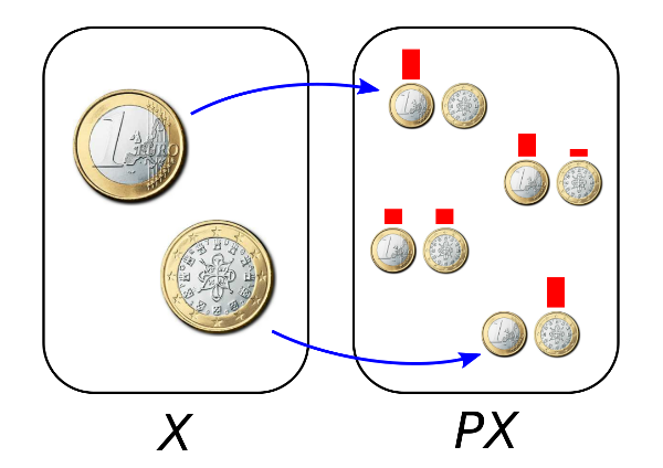
Let $X$ be a complete metric space. Among the measures of $P X$ there are some which are particularly simple: let’s call simple measures the ones of the form

$$p = \frac{1}{n} \, \big(\delta(x_1) + \dots + \delta(x_n)\big) ,$$

for points $x_1,\dots,x_n\in X$. These measures can be thought of as the empirical distributions coming from finite sequences $(x_1,\dots,x_n)$. It is well-known that simple measures are dense in $P X$. In other words, with the Kantorovich metric, we can approximate any probability measure $p\in P X$ by a sequence of simple measures.

Thanks to the choice of our category, we can express this density property in the language of category theory as a colimit. In particular, for each $n\in \mathbb{N}$, let $X^n$ denote the $n$-th cartesian power of $X$, equipped with the rescaled metric:

$$d\big( (x_1,\dots,x_n) , (y_1,\dots,y_n) \big) \coloneqq \frac{1}{n} \sum_{i=1}^n d(x_i,y_i) .$$

Let us now take a quotient space of $X^n$ with respect to permutations, effectively defining the space of $n$-tuples of elements of $X$ up to reordering. In rigor, we define the space $X_n$ to be the quotient space of $X^n$ under the action of the symmetric group $S_n$, with the quotient metric:

$$d\big( (x_1,\dots,x_n) , (y_1,\dots,y_n) \big)\coloneqq\min_{\sigma\in S_n} \frac{1}{n} \sum_{i=1}^n d(x_i,y_{\sigma(i)}) .$$

The spaces $X^n$ and $X_n$ are again complete metric spaces, objects of $CMet$. Now the density result, intuitively, says that $P X$ is in some sense the colimit over $n$ of the spaces $X_n$. To make this precise, we have to give the indexing category over which to take the colimit. So let $N$ be the category whose objects are nonzero natural numbers, and with a morphism $n\to m$ if and only if $n$ divides $m$. We can construct a functor $X_{-}\colon N\to CMet$ mapping the number $n$ to the space $X_n$, and the morphism $n\to n k$ (for $n,k$ natural numbers) to the function $X_n\to X_{n k}$ which copies $k$ times the sequence $(x_1,\dots,x_n)$:

$$(x_1,\dots,x_n) \mapsto (x_1,\dots,x_n,x_1,\dots,x_n,\dots,x_1,\dots,x_n) .$$

The construction is also functorial in $X$: given a map $f\colon X\to Y$ we get a map $X_n\to Y_n$ by just applying $f$ elementwise. The fact that simple measures are dense in $P X$ now reads as follows.

Theorem. The space of probability measures $P X$ can be expressed as the following colimit: $$P X = colim_{n\in N} X_n .$$

A similar statement can also be given using the $X^n$, without quotienting over permutations (see our paper for more details on this).

Monad structure arising from the colimit

We have seen that we can determine the functor $P$ in terms of the spaces of finite sequences $X_n$. The monad structure of $P$ can be also defined purely in terms of finite sequences, in a way which is quite close to how one uses integration in practice (at least, in the interpretation given above). Let’s see how. First of all, let $m$ and $n$ be natural numbers, and consider the elements of $(X_m)_n$, which are the sequences of sequences, in the form

$$((x_{1 1},\dots,x_{m 1}),\dots, (x_{1 n},\dots,x_{m n})) .$$

There is a map $E_{m,n}\colon (X_m)_n \to X_{m n}$ which we can think of as “removing the inner brackets”, or “flattening the array”:

$$((x_{1 1},\dots,x_{m 1}),\dots, (x_{1 n},\dots,x_{m n})) \; \mapsto \; (x_{1 1},\dots,x_{m 1},\dots, x_{1 n},\dots,x_{m n}) .$$

This map is already the “core” of the “averaging” map $P P X\to P X$ which gives the multiplication of the monad: the empirical distribution of the sequence

$$(x_{1 1},\dots,x_{m 1},\dots, x_{1 n},\dots,x_{m n})$$

is exactly the average of the empirical distributions of the sequences

$$(x_{1 1},\dots,x_{m 1}),\dots, (x_{1 n},\dots,x_{m n}) .$$

We can make the statement concrete by appealing to the universal property of $P$. It turns out that there is a unique map $E\colon P P X\to P X$ extending by continuity the maps $E_{m,n}\colon (X_m)_n \to X_{m n}$. This map is precisely the integration, and this way it is even defined without mentioning measure theory at all.

The fact that the resulting $E$ satisfies the monad axioms comes from the fact that the $E_{m,n}$ satisfy similar axioms, which can interpreted in terms of adding and removing brackets.

For example, for the analogue of the associativity diagram for the $E_{m,n}$, suppose we are given $m,n,k\in N$, and we consider a triple sequence, i.e. an element of $((X_k)_m)_n$ in the form

$$(((x_{1 1 1},\dots ,x_{k 1 1}), \dots , (x_{1 m 1},\dots ,x_{k m 1})),\dots,((x_{1 1 n},\dots ,x_{k 1 n}), \dots , (x_{1 m n},\dots ,x_{k m n}))).$$

We can first remove the innermost brackets to obtain

$$((x_{1 1 1},\dots ,x_{k 1 1}, \dots , x_{1 m 1},\dots ,x_{k m 1}),\dots,(x_{1 1 n},\dots ,x_{k 1 n}, \dots , x_{1 m n},\dots ,x_{k m n}))$$

and then remove the remaining inner brackets to obtain

$$(x_{1 1 1},\dots ,x_{k 1 1}, \dots , x_{1 m 1},\dots ,x_{k m 1},\dots,x_{1 1 n},\dots ,x_{k 1 n}, \dots , x_{1 m n},\dots ,x_{k m n}).$$

Or we can first remove the middle-level brackets to obtain

$$((x_{1 1 1},\dots ,x_{k 1 1}), \dots , (x_{1 m 1},\dots ,x_{k m 1}),\dots,(x_{1 1 n},\dots ,x_{k 1 n}), \dots , (x_{1 m n},\dots ,x_{k m n}))$$

and then remove the remaining inner brackets to obtain

$$(x_{1 1 1},\dots ,x_{k 1 1}, \dots , x_{1 m 1},\dots ,x_{k m 1},\dots,x_{1 1 n},\dots ,x_{k 1 n}, \dots , x_{1 m n},\dots ,x_{k m n}) .$$

In the two cases the result is the same. This, after taking the colimit, implies that the associativity diagram for $E:P P X\to P X$ commutes.

In particular, the functors $X\mapsto X_n$ (and also $X\mapsto X^n$) are said to form a graded monad. For the theory of graded monads see the paper

• Fujii, Katsumata and Melliès, Towards a formal theory of graded monads. In: Jacobs B., Löding C. (eds) Foundations of Software Science and Computation Structures. FoSSaCS 2016. Lecture Notes in Computer Science, vol 9634. Springer, Berlin, Heidelberg. (pdf)

In general, the statement is that under some mild conditions, the colimit of a graded monad is a (traditional) monad.

Theorem. The functor $P$ can be equipped with a unique monad structure $(P,E,\delta)$ induced by the maps $E_{m,n}$ and the universal property of $P$.

Algebras

We have said above that algebras of a probability monad tend to look like convex spaces. This is the case for the Kantorovich monad too. In particular, algebras have to be objects of our category, complete metric spaces. An ideal candidate is then closed convex subsets of Banach spaces, since they are complete metric spaces, they are convex, and the convex and metric structures interact nicely with each other. This turns out to be indeed the case:

Theorem. The algebras of the Kantorovich monad are exactly the closed convex subsets of Banach spaces, with the induced metric and convex structure.

The proof of this statement relies on the colimit characterization above, and on previous work of Tobias with Valerio Capraro, which in turn is based on the celebrated Stone’s theorem for convex structures. More information about this can be also found in David Corfield’s post here on the Café about convex spaces. Therefore, the Kantorovich monad gives a framework for treating categorically random variables with values in Banach spaces.

Further questions and reading

Some questions arise from the construction of this monad.

• Is there a way of obtaining the law of large numbers, or a related result, as a category-theoretical statement?
• Are there generalizations to Lawvere metric spaces?

A more algebraic question is the following.

• Which other monads arise as colimits of graded monads, how general is the construction?

If you want to know more, there are the papers of Tobias and myself on the topic (here, here, and here), my PhD thesis (pdf), more work is still in progress. There is also Tobias’ recent talk at MIT. Tobias and I are also working on a project at the Applied Category Theory Adjoint School this year, together with Nathan Bedell, Carmen Constantin, Martin Lundfall, and Brandon Shapiro. The project partly involves the Kantorovich monad, and there will be posts about it on this blog in the coming weeks. So, stay tuned!