Diversity and the Mysteries of Counting
Posted by Tom Leinster
.")
Back in 2005 or so, John Baez was giving talks about groupoid cardinality, Euler characteristic, and strange objects with two and a half elements.
I saw a version of this talk at Streetfest in Sydney, called The Mysteries of Counting. It had a big impact on me.
This post makes one simple point: that by thinking along the lines John advocated, we can arrive at the exponential of Shannon entropy — otherwise known as diversity of order .
Background: counting with fractional elements
Consider a group acting on a set , both finite. How many “pieces” of are there, modulo ?
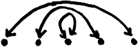
The first, simple, answer is , the number of orbits. For example, in the action of on the five-element set shown in the diagram above, this gives an answer of .
But there’s a second answer: , the cardinality of divided by the order of . If the action is free then this is equal to , but in general it’s not. For instance, in the example shown, this gives an answer of .
The short intuitive justification for this alternative answer is that when counting, we often want to quotient out by the order of symmetry groups. For example, there are situations in which a point with an -action deserves to count as only elements. John’s slides say much more on this theme.
This second answer also fits into an abstract framework.
Every action of a group on a set gives rise to a so-called action groupoid . Its objects are the elements of , and a map is an element such that . Equivalently, it’s the category of elements of the functor corresponding to the group action.
There is a notion of the cardinality of a finite groupoid . And when you take the cardinality of this action groupoid, you get exactly . That is:
In summary, the first answer to “how many pieces are there?” is , and the second is .
Now let’s do the same thing with monoids in place of groups. Let be a monoid acting on a set , and assume they’re both finite whenever we need to. How many “pieces” of are there, modulo ?
Again, the obvious answer is . Here is again the set of orbits. (You have to be a bit more careful defining “orbit” for monoids than for groups: the equivalence relation on is generated, not defined, by if there exists such that .)
And again, there’s a second, alternative answer: .
The abstract framework for this second answer is now about categories rather than groupoids. Every action of a monoid on a set gives rise to an action category . It has the same explicit and categorical descriptions as in the group case.
There is a notion of the Euler characteristic or magnitude of a finite category . It could equally well be called “cardinality”, and generalizes groupoid cardinality. And when you take the Euler characteristic of this action category, you get . That is:
So just as for groups, the first and second answers to “how many pieces are there?” are and , respectively.
How diversity emerges
Take a surjective map of sets . We’re going to think about two structures that arise from :
The monoid of endomorphisms of over (that is, making the evident triangle commute). The monoid structure is given by composition.
The set of all endomorphisms of . We could give this a monoid structure too, but we’re only ever going to treat it as a set.
The monoid acts on the set on the left, by composition: an endomorphism of followed by an endomorphism of over is an endomorphism over . (The fact that one of them is over does nothing.)
So, how many pieces of are there, modulo ?
The first answer is “count the number of orbits”. How many orbits are there?
It’s not too hard to show that there’s a canonical isomorphism
where the right-hand side is the set of functions . It’s a simple little proof of a type that doesn’t work very well in a blog post. You start with the fact that composition with gives a map and take it from there.
So assuming now that and are finite, the number of orbits is given by
That’s the first answer, but while we’re here, let’s observe that this equation can be rearranged to give a funny formula for the cardinality of :
The second, alternative, answer is that the number of pieces is
What is this, explicitly? Write the fibre as . Then
and since , this gives
as our second answer.
Now here’s the punchline. The first answer gave us a formula for the cardinality of :
What’s the analogous formula for the second answer? That is, in the equation
what goes on the left-hand side?
Well, it’s
We can simplify this if we write . These numbers are nonnegative and sum to , so they amount to a probability distribution
The formula for “?” then simplifies to
And this is nothing but the exponential of Shannon entropy, also called the diversity or Hill number of order .
In conclusion, if we take that first-answer formula for the cardinality of —
— then its second-answer analogue is a formula for the diversity of —
And this is yet another glimpse of an analogy that André Joyal first explained to me one fateful day in Barcelona in 2008: exponential of entropy is a cousin of cardinality.
Re: Diversity and the Mysteries of Counting
Beautiful!
I learned about the diversity of order 1 while reading Shannon’s seminal paper and I always liked it more than the entropy because it has the nice interpretation as “the probability of a typical event”, and because it has the form of the “endomorphism number of the probability distribution” if you squint and pretend that everything you can do in the biclosed equipment of spans works for good ol’ matrices as well. I mentioned this to David Spivak at some point and he came back and told me about this counting endomorphisms story which requires significantly less squinting, but still had a pesky division where it shouldn’t be.
This is a great explanation of why that pesky division really should be there!
This makes me wonder: what other quantities and ways of doing things from basic information theory and probability theory can be described “objectively” with the combinatorics of surjections of finite sets like this?