The n-Category Café

Application: Intrusion detection in computer networks

The revolution of the internet, short for internetwork, has made our fantasies of space travel and teleportation a near reality. As you are reading this blogpost, your computer is transferring messages to other computers possibly thousands of miles away, using common communication protocols like the Transmission Control Protocol (TCP). These messages contain the data that is shown in your browser including the internet protocol (IP) address you are receiving the data from. For example, your laptop or desktop computer has just received the HTML describing the layout and content of you words you are reading on the screen from another computer at the University of Texas (as indicated by the golem.ph.utexas.edu hostname).

Aside from TCP/IP, there are other types of communication protocols that you can use to pass different messages to other computers. Suppose you are interested in logging into another computer from your laptop or desktop without walking all the way over to its location. Well you can do this via the remote desktop protocol (RDP) to forward the target computer’s desktop screen, or you can use a secure shell (SSH) connection to log into the computer from a terminal. A secure shell (SSH) connection may give you read and write access to a computer’s file system, applications, services via a terminal. If you find that a bad actor has gained access to your system via SSH, you may find yourself in a precarious situation. A recent example of this involves the failure to filter SSH connections in TP-Link Archer A7 AC1750 routers. If you own this as your home or enterprise router, it may be possible gain access to your personal computer from a remote location without your knowledge.

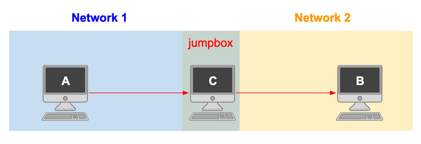
Evidently, this powerful access could lead to sensitive data exposures or malicious attacks on critical computers. Most enterprise information technology departments mitigate this risk by sanctioning certain machines onto isolated networks via firewalls or accessibility lists. This means that only a subset of the computers existing in the enterprise will have the ability to communicate with each other via TCP/ICP, SSH, and other protocols. If you are working on your personal laptop but need to gain access to sensitive data existing on a computer on the isolated network, you may need to “pass through” a computer that you have access to in order to gain access to the highly restricted machine. This “pass through” computer is often called a jump box or jump host.

Intrusion detection

Now imagine you are a network administrator of a hospital’s IT department who has just discovered that a disgruntled employee has chosen to SSH into a machine containing patient healthcare data with a desire to delete or tamper with these documents. There are thousands of machines on your enterprise network so you cannot simply shutdown the whole network because there are some essential for patient care. One way to combat this action is to identify the computer that they are using as their jump box and shut it down. You know the IP address of the employee’s computer, you know the IP address of the machine containing the patient data, and you have a suspicion about which jump box the employee is using. Before taking action, you want to validate that the employee’s computer does in fact have access to the patient data via the specific jump box. Your question then becomes can computer A access computer B via computer C?

SSH Connection Logs

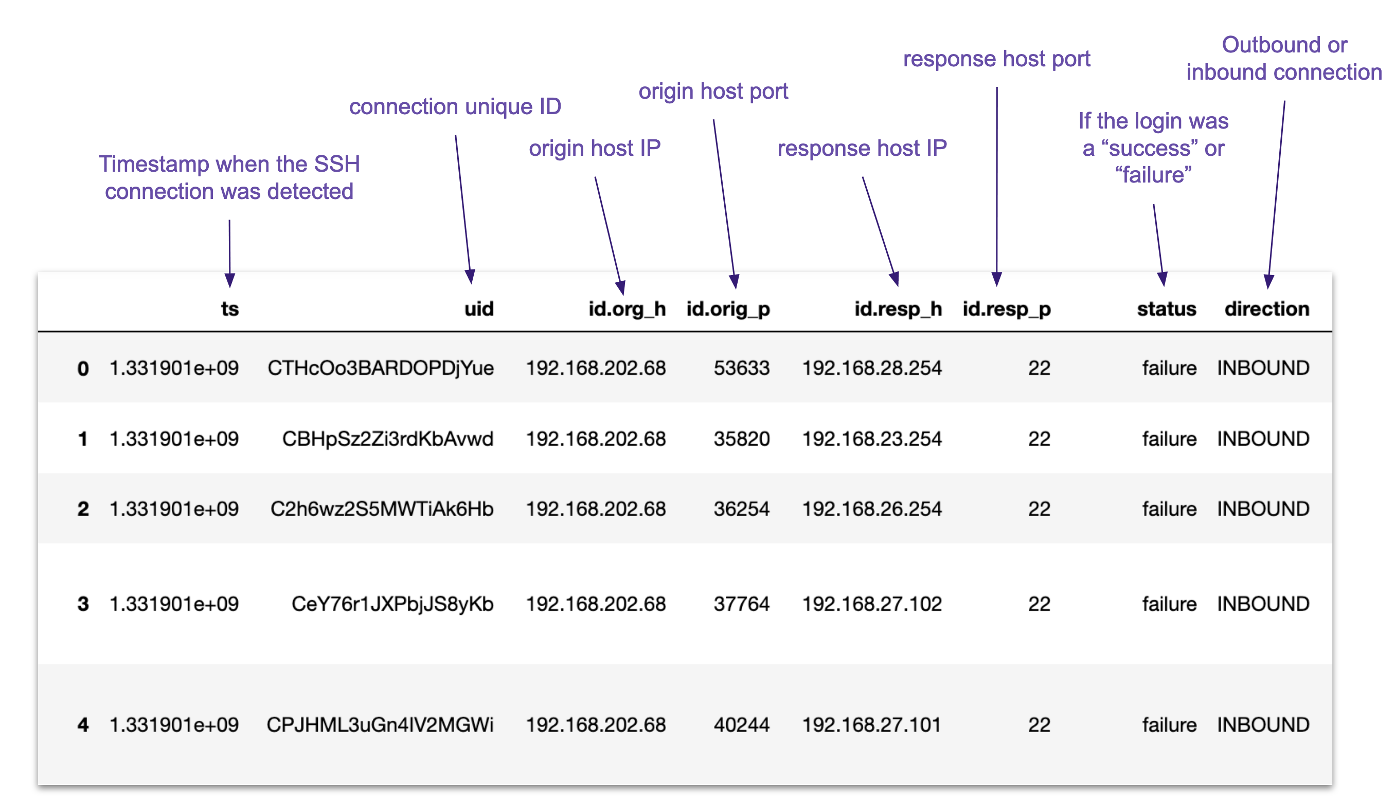
To solve this problem we can do a network scan using tools like Zeek to capture all SSH connections occuring within a given duration of time. Luckily, we have historical SSH connection logs for our hospital IT infrastruture! These logs are comma-separated text files that contain the IP and port information about the source machine and target machine for every SSH connection.

A digraph can be generated from this description.

Definition (digraph): A digraph is a pair of sets, $(V, E)$, with $E \subseteq (V \times V)$. The elements of $V$ are vertices and the elements of $E$ are edges. For $e = \{(v_i, v_j) | v_i, v_j \in V\}$, where $v_i$ is the source of $e$ and $v_j$ is the target of $e$. The source and target can be captured using maps $s: E \rightarrow V$ and $t: E \rightarrow V$, respectively.

Example (Connection Logs): A digraph for connection logs can be instantiated by providing the set of unique machine IPs as $V$ and the set of connections, denoted by every row in the log, as $E$.

Notice that the set of unique host machine IPs exist in the category $\mathbb{FinSet}$. A full definition of $\mathbb{FinSet}$ can be found in nlab.

Definition (digraph category $\mathbb{Dgr}$): The category $\mathbb{Dgr}$ has digraphs as objects, and a morphism from the digraph $(V, E)$ to the digraph $(V', E')$ is a function $f: V \rightarrow V'$ such that $\{f(v), f(w)) \in E' | (v, w) \in E\}$. See nlab.

Example

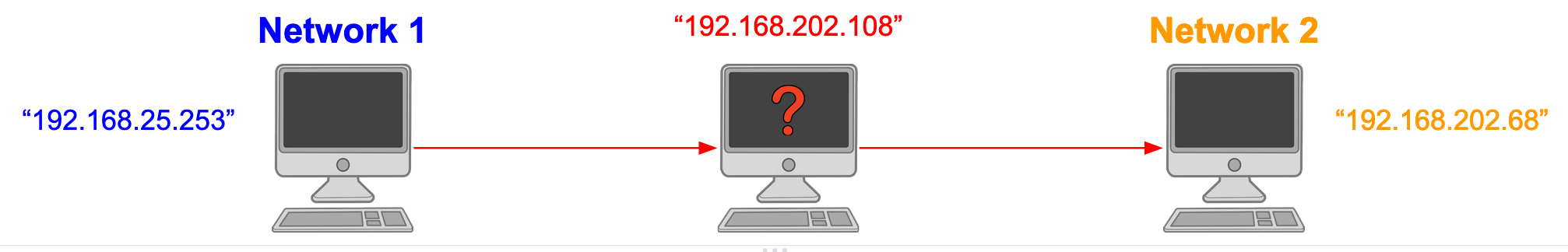
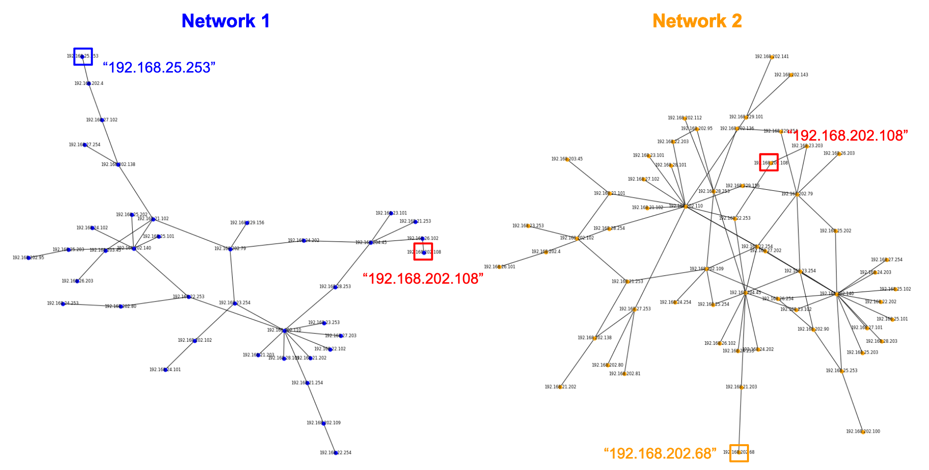
We can simulate this problem using SSH connection logs derived from a dataset hosted by SecRepo by Mike Sconzo. This dataset captures logs for a single network. The dataset has been sampled to generate two separate sub-digraphs with at least one common node, which will emulate our jump box. Note: This permits both digraphs to have more than one overlapping node. This characteric further emphasizes the value of the structured cospan method. We name the networks produced by the two digraphs as Network 1 (A) and Network 2 (B).

In our example, we can identify a source IP in our dataset as being "192.168.25.253", our target IP as being "192.168.202.68", and our jump box IP as being "192.168.202.108".

Using this information, we can set-up our code in Julia to be:

# Julia
import JSON
datasetA = JSON.parsefile("datasetA.json")
datasetB = JSON.parsefile("datasetB.json")

source_ip = "192.168.25.253"
target_ip = "192.168.202.68"
jumpbox_ip = "192.168.202.108"

Structured cospans

The structured cospan construction was defined by John Baez and Kenny Courser to provide a formal way to compose open systems. In this context, an open system is a combinatorial object (i.e. set, graph, …) that contain the notion of having inputs or outputs. The basic ingredients to making a structured cospan include: * a cospan in a “less structured” category * a decoration functor ($F$) to a “more structured” category

To formulate this problem as a structured cospan, we can say our “more structured” category is $\mathbb{Dgr}$ and our “less structured” category is then $\mathbb{FinSet}$. This means that the cospan exists in $\mathbb{FinSet}$. Semantically, a leg in the cospan means that we are marking a host IP in one network as being significant. More specifically, the following functions are defined:

$$source: S_{IP} \rightarrow S_{IP}$$
$$jumpbox: S_{IP} \rightarrow S_{IP}$$
$$target: S_{IP} \rightarrow S_{IP}$$

The decoration functor $F: FinSet \rightarrow Dgr$ takes a set of IPs to a digraph according to the respective log entries. This provides us with the following maps:

$$F(A): FinSet(A) \mapsto Dgr(A)$$ $$F(B): FinSet(B) \mapsto Dgr(B)$$

We understand our functor, $F$, to be a left adjoint and, therefore, can construct the corresponding finite sets for each dataset from it’s connection log representation using a right adjoint. The right adjoint functor is defined by get_IP(dataset, fields) below:

# Julia
function get_IP(dataset::Array, fields::Array{String})
    global ip = []
    for entry in dataset
        for field in fields
            global ip
            push!(ip, entry[field])
        end
    end
    return unique(ip)
end

# Get uniq IPs in each dataset
ip_A = get_IP(datasetA, ["id.org_h", "id.resp_h"])
ip_B = get_IP(datasetB, ["id.org_h", "id.resp_h"])

As aforementioned, we can loop through connection logs for each dataset to construct two digraphs which will serve as the decoration upon the cospan apexes. Using the Catlab library, we can instantiate two structured cospans shown below:

# Julia
using Catlab
using Catlab, Catlab.Theories, Catlab.Graphs,
Catlab.CategoricalAlgebra, Catlab.CategoricalAlgebra.FinSets, Catlab.Graphics

const OpenGraphOb, OpenGraph = OpenCSetTypes(Graph, :V);  #  (StructuredCospanOb{L}, StructuredMulticospan{L})

function build_cospan_security(ip_list::Array{Any,1}, conn_log::Array{Any,1}, input_ip::String, output_ip::String)
    # get index of desired IPs
    input_index = findall(x->x==input_ip, ip_list) 
    output_index = findall(x->x==output_ip, ip_list) 

    num_nodes = size(ip_list)[1]
    graph = Graph(num_nodes)

    # For each entry, record edge between IPs
    for entry in conn_log
        s = entry["id.org_h"] # source IP of SSH connection
        t = entry["id.resp_h"] # target IP of SSH connection

        s_index = findall(x->x==s, ip_list)[1] # there should only be 1
        t_index = findall(x->x==t, ip_list)[1] # there should only be 1

        add_edge!(graph, s_index, t_index)
    end

    # Create structured multicospan (L-form), i.e. structured cospan
    cospan = OpenGraph(graph, FinFunction(input_index, num_nodes), FinFunction(output_index, num_nodes))  # (apex, leg, leg)
end

cospan_A = build_cospan_security(ip_A, datasetA, source_ip, jumpbox_ip);
cospan_B = build_cospan_security(ip_B, datasetB, jumpbox_ip, target_ip);

This gives us structured cospans that look like–

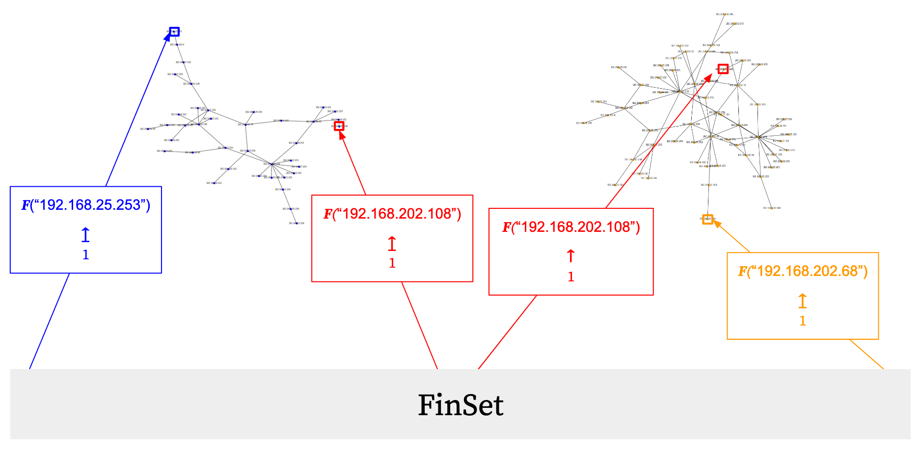
An important thing to note is that, in the Julia code, the IPs have been indexed such that we can refer to them as integers when constructing our graph. This is required by the current implementation of Graph in Catlab.

Now that we have our cospans set-up we can consider a few approaches to answering the question of whether the two computers can communicate.

Approach 1: Using non-disjoint union

The most common approach to evaluating connectivity in computer networks is to vertically stack the connection logs (i.e. take the non-disjoint union), generate a graph, and check if two IPs are one connected component. This requires the additional step of checking all the paths from computer A to computer B to see if any of them pass through the node for computer C. This computation would scale proportionally to the size of the graph, which is not ideal. The resulting graph would look like this.

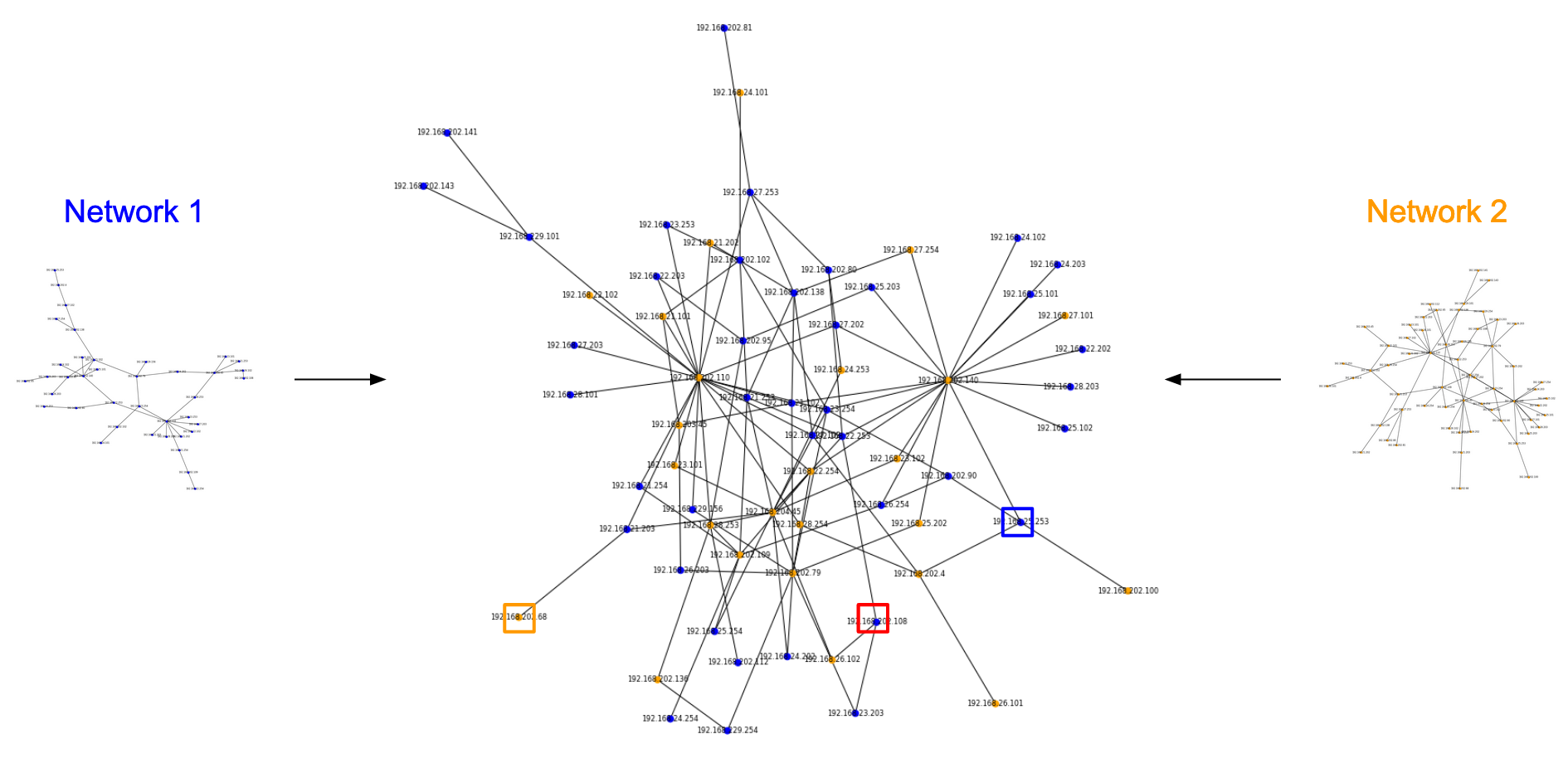
Note: This is just the same as taking the pushout where the span is the intersection of the finite sets of IPs in both networks.

Approach 2: Using structured cospan

Alternatively, because we have chosen a structured cospan formulation, this allows us to choose what to identify as our common leg, or our span for our pushout. For our example, this would just be the jump box IP address.

In order for this to work another map needs to be defined to finish up structured cospan construction. Namely,

$$F(A +_{j} B): FinSet(A +_{j} B) \mapsto Dgr(A +_{j} B)$$

To ensure that F(A +{j} B) adheres to the coherence maps, we can add suffixes to the IP names according to the dataset they belong to, i.e. _A and _B, but ignore this step for IP names belonging to the jump box. Taking the union of these data entries will exactly provide the pushout, F_{A +{j} B}.

Luckily for us, the logic to take care of the pushout for graphs is implemented in Catlab. We can simply compose the two cospans and the apex of the new cospan will be the pushout of the two apex digraphs.

# Julia
pushout = compose(cospan_A, cospan_B);

Connectivity via coequalizers

The last step is to figure out if the source IP and target IP are connected via our jump box IP. We can do this by computing a coequalizer on the apex of the pushout.

Definition (coequalizer) A coequalizer in category $\mathbb{C}$ is a colimit of parallel morphisms $f, g$ in $\mathbb{C}$.

In Catlab, the coequalizer for graphs is implemented underneath connected_components

# Julia
components = connected_components(apex(pushout));

To complete the analysis, we simply need to look at our connected components and check if our source and target IPs are connected. Due to the definition of the pushout, we guarantee that the only way those machines can be connected is via our jump box IP. An example implementation for checking for this is shown here:

# Julia
# Derive our source and target IP indices in apex graph
source_index = findall(x->x==source_ip, ip_A)[1]
jumpbox_index = findall(x->x==source_ip, ip_A) 
target_index = size(ip_A)[1] + findall(x->x==target_ip, ip_B)[1] - size(jumpbox_index)[1]

# Check connectivity between source and target IP
for c in components
    if (source_index in c) & (target_index in c)
        print(source_ip, " is connected to ", target_ip, " via jumpbox IP ", jumpbox_ip)
    end
end

---

192.168.25.253 is connected to 192.168.202.68 via jumpbox IP 192.168.202.108

We have successfully used structured cospans to solve the problem. We can now shut down that jump box and save the hospital!

Conclusion

In conclusion, we have walked through an example in which composing commonly used open systems, namely computer networks, can be described using structured cospans. What we found to be the most powerful feature of structured cospans is the ability to choose the span in which we want to quotient over in our composition.

This was nicely put in Seven Sketches of Compositionality, Chapter 6.2.3:

“The pushout construction, however, is much more general [as opposed to nondisjoint union]; it allows (and requires) the user to specify exactly which elements will be identified.”

It gives us the power to decide what to glue, instead of gluing the whole thing! There are many other examples in engineering and data science where fine-tuning the composition of combinatorial objects would save a lot of time in computation, such as in computing reachability in robot motion configuration spaces and computing connectivity of social media networks. We hope that many more examples applying the structured cospan method can be brought to the fore.