How to Apply Category Theory to Thermodynamics
Posted by Emily Riehl
.")
guest post by Nandan Kulkarni and Chad Harper
This blog post discusses the paper “Compositional Thermostatics” by John Baez, Owen Lynch, and Joe Moeller. The series of posts on Dr. Baez’s blog gives a more thorough overview of the topics in the paper, and is probably a better primer if you intend to read it. Like the posts on Dr. Baez’s blog, this blog post also explains some aspects of the framework in an introductory manner. However, it takes the approach of emphasizes particular interesting details, and concludes in the treatment of a particular quantum system using ideas from the paper.
Thermostatics is the study of thermodynamic systems at equilibrium. For example, we can treat a box of gas as a thermodynamic system by describing it using a few of its “characteristic” properties — the number of particles, average volume, and average temperature. The box is said to be at equilibrium when these properties do not seem to change — If you were to take a thermometer and measure the temperature of the box at equilibrium, the thermometer’s reading should not change over time.
The paper “Compositional Thermostatics” introduces a framework in category theory for doing thermostatics. If the properties of some thermodynamic systems can be represented as a convex space, and given an entropy function for these systems, this framework can be used to compute the entropy function of a new system formed by coupling these systems together somehow.
In this post, we will offer an interpretation of this framework, and then apply the framework to a non-trivial problem in quantum mechanics involving density matrices. In other words, we will attempt to respond to the following questions, in order: How should a scientist think about this framework? Why and how would a scientist use this framework?
The importance of interpretation
If we wanted to, we could use the framework unthinkingly, as follows:
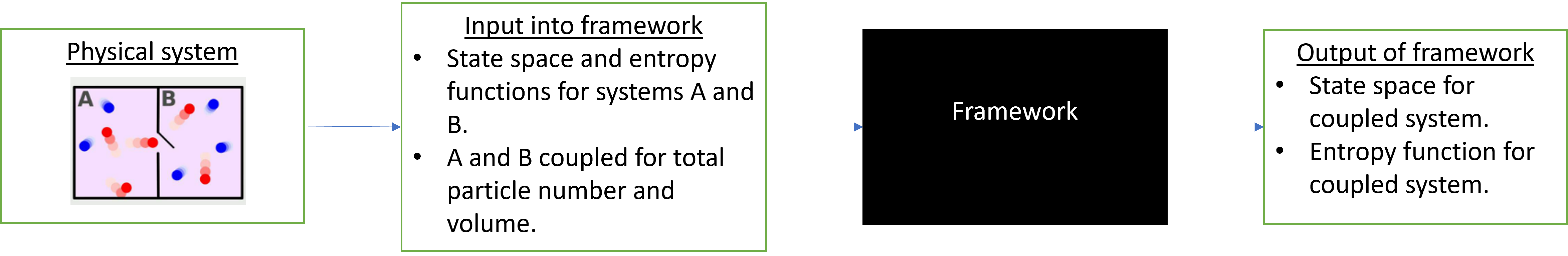
Figure 1
In that case, the only “interpretive” work we’d have to do would be
- Figure out how to mathematically represent the physical systems using a convex state space and entropy function.
- Understanding what the output of the framework means.
For most simple thermodynamic systems, this would work pretty well, because the framework was built keeping these systems in mind. However, we would then lose out on the really interesting part — the inner workings of the framework itself.
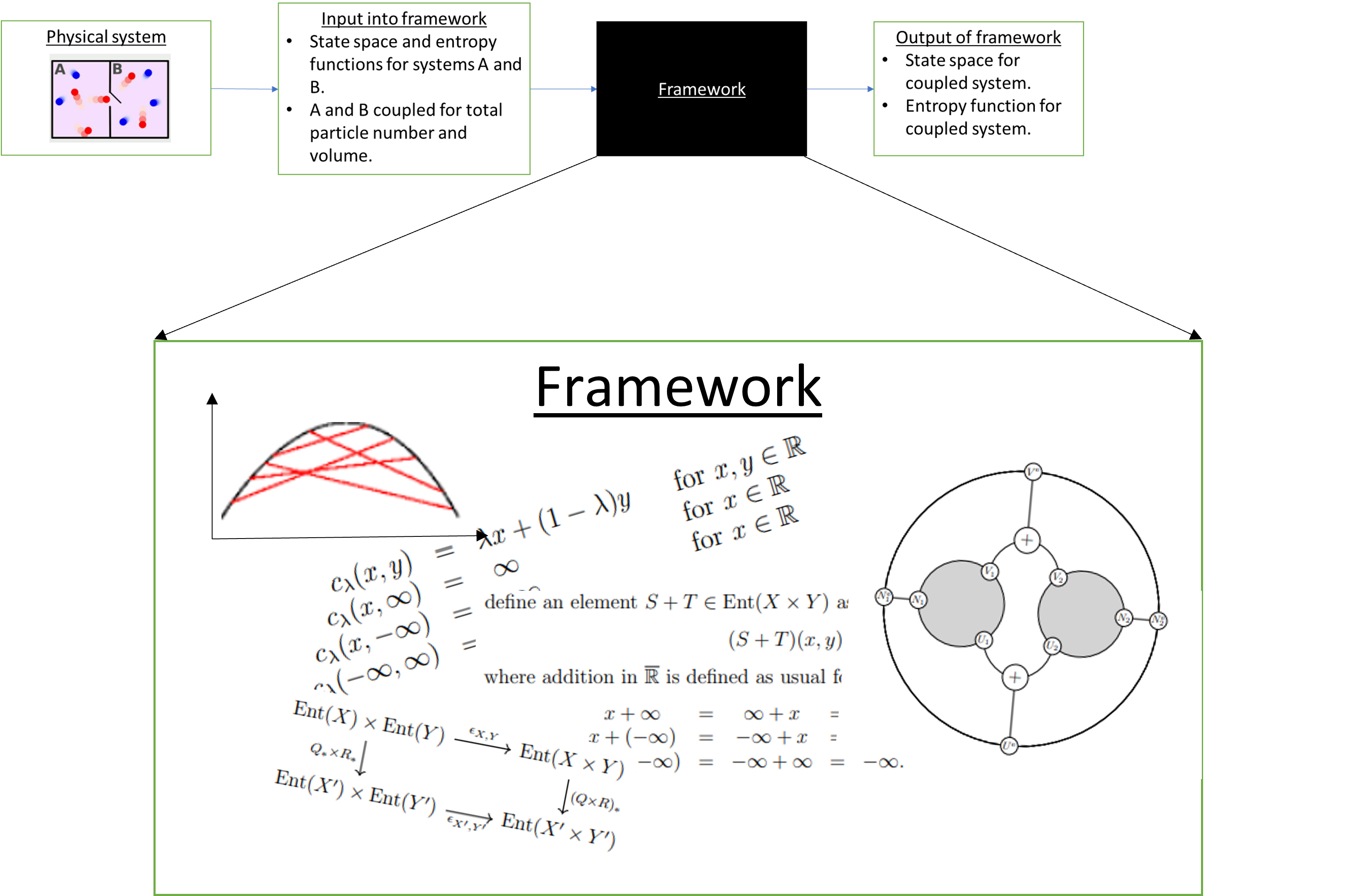
Figure 2
An “interpretation” of what all this machinery is doing offers an interpretation of the theory of thermostatics itself. I think this is what makes applied category theory really interesting. It is as much about figuring out how to think about a subject such as thermodynamics as building computational tools to study it. I hope that existing knowledge of category theory may then push our understanding of the subject even further through the interpretations we attach to the frameworks we build.
Setting up a thermostatic system: State spaces and entropy
When we describe the possible states of a thermodynamic system using points in set , such as using points in to refer to the number of particles, volume, and temperature of a box of gas, we call the “state space” of the physical system we are studying.
An entropy function associated with state space is a function , where is the extended reals. Entropy can have many interpretations. According to the second law of thermodynamics, if the system can change from one state, represented by point , to another state, represented by , then . When dealing with certain thermodynamic systems, we may extend this to the maximum entropy principle: A thermodynamic system with state space will evolve to a subset of where the entropy function is maximized (a set of equilibrium states), and remain there. Imagine a stretched rubber band pulling itself back to its original shape. We might say that the entropy of the rubber band is maximized when in the state of its original shape.
Thermodynamic systems are often studied under the effects of various constraints that limit their state space to a subset of the full space. For example, suppose you begin with two tanks of incompressible fluid, with tank #1 described by its energy and tank #2 similarly described by . Physics tells us that if a valve is opened allowing free exchange between these boxes, the new thermodynamic system is described by the sum of their energies due to energy conservation. The state space of the new system is .
When we consider the combined system, which we will call , made from tanks called and , each point in the state space of corresponds to a whole range of states of and — An energy of for corresponds to , where a point in represents the state of together with a state of .

Figure 3
The way to write this in the framework for thermodynamic systems in general as follows: Suppose you build a system with state space from system with state space . You can describe how is built from using a relation , where . In Figure 4, point represents a state of . If we observe , it could mean the system is at any state in the blue region. The knowledge of what exactly that blue region looks like comes from , which carries information about how exactly is formed from . Thus, for now, we may think of systems as morphisms in the category — The category of sets and relations.
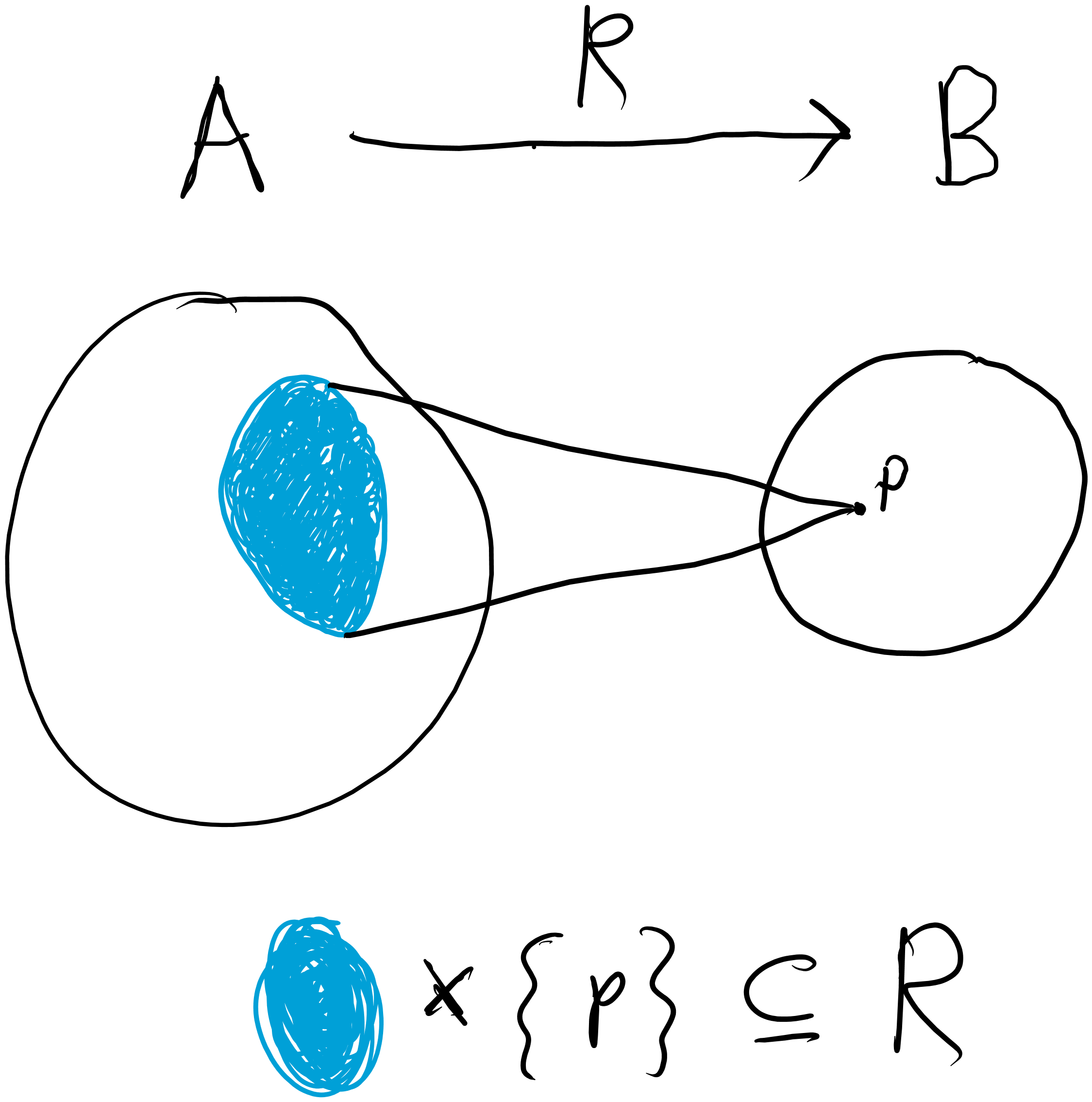
Figure 4
So, knowing the entropy function on , and knowing , can we calculate the entropy for system with state represented by ? This is possible using our understanding of how physical systems behave: We can interpret the maximum entropy principle to say that if a system described by is observed at a state respresented by , then we expect it to exist at a point in the blue region with maximum entropy. Thus, the entropy function for the new system is
A more nuanced interpretation of the maximum entropy principle is that the system can and will evolve from any point in the blue region to a subset of the blue region with maximum entropy. More generally, since many entropy functions may exist for different systems described by the same state spaces, such as the tanks of fluid , , and all having state space in the earlier example, we might interpret the maximum entropy principle more strongly as follows: A thermodynamic system can evolve from any state corresponding to a point in the blue region to any other state with its point in the blue region, and additionally, the system will evolve to a collection of states corresponding to a subset of the blue region that maximizes entropy and remain there.
In the paper’s framework, we deal with sets equipped with “canonical paths” between points: For points and in state space , we have that follows certain rules:
Writing for , And where and ,
By requiring that the state spaces be convex (ie. every two points in state space is associated with a path ) and that relations be convex relations, we guarantee that for any , all “blue regions” of are convex as well. Thus, we choose to work in rather than . In this framework, if a subset of a state space is convex, then every state of the system in that subset is accessible from every other state.
An interpretation of this may be that the paths represent thermodynamic processes that can occur. If exists for some , then is accessible from by a known process, parameterized by . These are not necessarily the only allowed processes. But they are sufficient to describe which states are accessible from which others. This interpretation has some limitations. For one, the framework does not allow in general for blue regions that are just the range of for some — is not necessarily convex, but a process from to would imply a process from to for some , .
Thus, we now have a full description of what should constitute a thermostatic system in the framework: A convex state space for the system of interest, convex relation describing how is constructed from some system with state space , and an entropy function . If the system is used to build itself (ie. we are studying system on its own), let and , so . This says the entropy function for is the entropy function for .
Properties of entropy: Extensivity and concavity
The entropy function is not arbitrary. Two properties of entropy other than the maximum entropy principle that commonly appear are “extensivity” and “concavity”. There are thermodynamical theories which first assume extensivity and then prove concavity for certain classes of systems, but we assume both of these properties immediately and build them into the framework.
Extensivity is the property of how entropy functions of systems are composed when those systems are put together. It means the entropy of two systems together is the sum of the entropies of the individual systems. In the example of the tanks of incompressible fluid, if the entropy of is and the entropy of is , then the entropy of the tanks coupled together is . It is a prescription for the entropy function of a coupled system given the entropy functions on its individual components. This is built into the framework and is explained later in this blog post in the section on operads.
Concavity is a property that limits the shape entropy functions can have. An entropy function is concave if for all , . Then, having the following convex structure on the extended reals,
forces certain shapes for the allowed entropy functions:
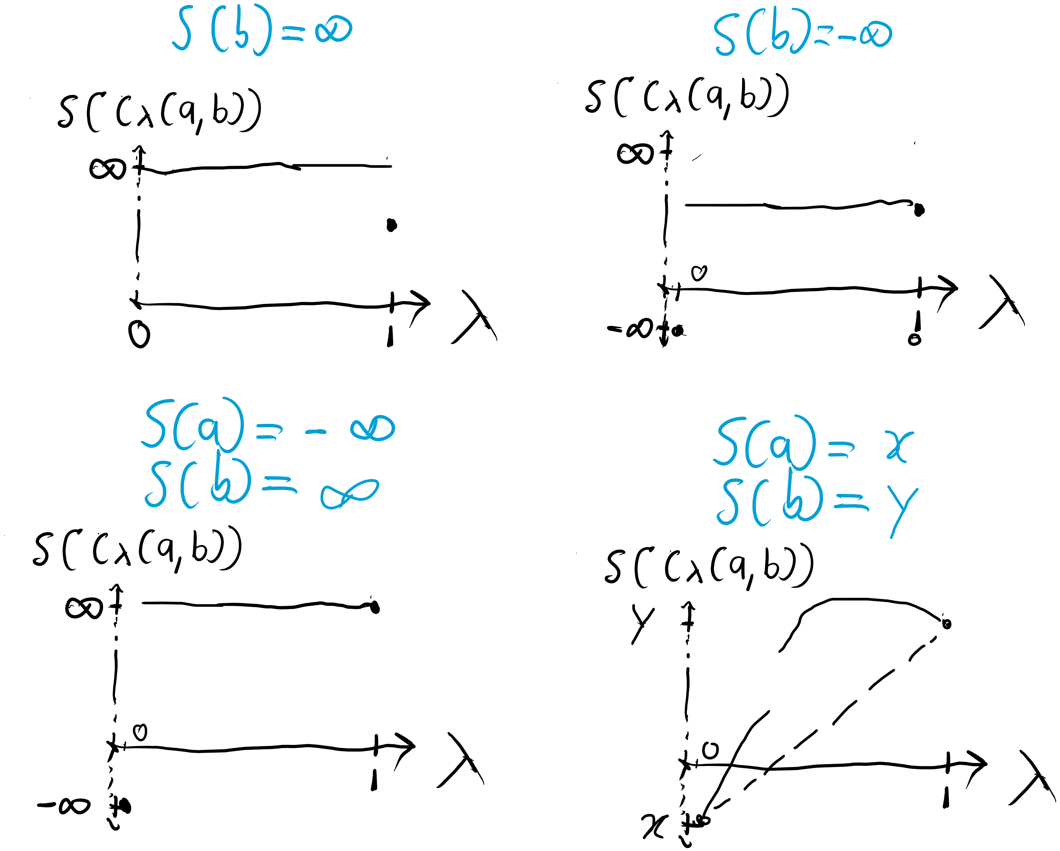
Figure 5
While concavity of entropy is a property of many common thermodynamic systems, it has some limitation. In some theoretical foundations for thermodynamics, such as that in the book “Statistical Mechanics of Lattice Systems: A Concrete Mathematical Introduction” by Sacha Friedli and Yvan Velenik, concavity of entropy is not immediately assumed, and rather arises out of certain properties of the lattice systems they deal with and the extensivity of entropy.
Mathematical machinery: Functors and operads
The functor
The functor is defined as follows:
- For convex space , takes to the set of entropy functions on , which is a an object in .
- For morphism , is a morphism . For entropy function , we define
Thus, the maximum entropy principle is built into this framework.
When we say is a functor, we mean that it has certain nice properties: It preserves identity morphisms and compositionality. Identity preservation means that for an unconstrained system, represented by , and given an entropy function on the system, the entropy function for the new system should still be . This is of course reasonable. Preserving compositionality means that given a series of relations , and an entropy function on , we have an equivalence between
- “Building” the entire system and calculating its entropy function.
- Calculating the entropy function of the system based on the entropy functions for each component of the system considered one at a time, ie. , then , …, then finally .
This ensures works consistently for all state spaces and relations. We will never have a situation where computing the entropy function for one way will give a different result from computing it any other way.
Because they’re everywhere in mathematics, we know a lot about functors in general in category theory. Thus, using functors in the framework also suggests opportunities to apply all our knowledge of category theory to deepen our interpretation of the framework.
Operads
Once again, I have been lying. The places we do thermostatics aren’t and , but rather and — the operads built over and . We simply use operads as a type of structure, like a category, where we can have state spaces and systems made from those state spaces represented by operations (the operad name for morphisms) between them.
The special thing about operads is that operations can take “inputs” from multiple types. For categories, we represent the morphisms from object to object as . For operad , we represent the operations from types to as . We can also compose operations
Because and are symmetric monoidal categories (with a notion of tensoring objects together and some “obvious” symmetries), there are “obvious” operads we can build from them.
For a symmetric monoidal category with tensor product , we can construct as follows:
- The types in are exactly the objects of .
- For types , operations of are exactly the morphisms .
- For operations The composition of and is , ie. , defined as
We now demonstrate how this is applied to and .
The tensor product of is the convex product defined as follows: For convex spaces , (formed from sets also called and ) and convex structures defined by and respectively, is given by the set and the convex structure defined by . The tensor product of is just the set product, which we will also call for simplicity. The meaning of will be clear from context.
Thus, the types of are convex spaces and elements of are convex relations, in particular the convex subsets of . A convex relation represents a way of coupling together the systems represented by state spaces to form the system represented by state space . The types in operad are sets and elements of are the functions from to .
The symmetric monoidal structure of has certain symmetries that can be interpreted to state that
- Coupling thermodynamic system to thermodynamic system is equivalent to coupling system to system — The isomorphism “braiding” implies that and can represent the same couplings of systems.
- Coupling thermodynamic system to system and then coupling that new system to is equivalent to coupling to system and then coupling to that new system — The isomorphism “associator” lets be written unambiguously.
Suppose we have a system with state space built from , a system with state space built from , and a system with state space built from and .
By itself, the category does not have the right structure to make our framework functional for coupling multiple systems in an elegant way. In , we could build , , and , but there is no prescription in the framework for how to compose with both and . We would have to build the system all at once “by hand”, with relation calculated from , , and .
The operadic approach, on the other hand, has the process of getting from , , and built into it through how composition is defined. Using , the process of coupling to form and to form , and then coupling and to form would look like this:
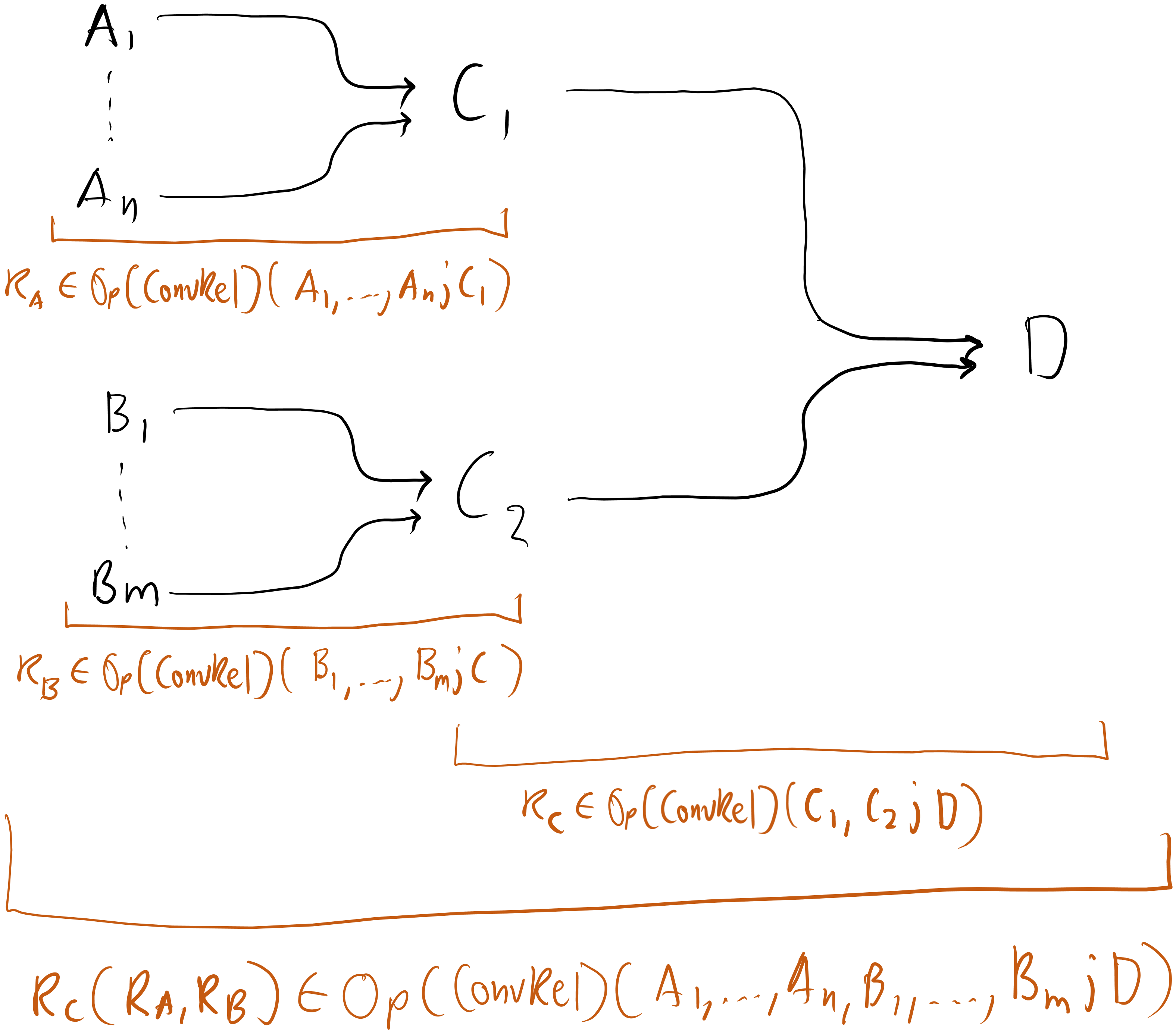
Figure 6
Here, each group of arrows represents a relation. Much more intuitive and elegant.
The work we did in was still important, because the functor we defined can be used to define a similar “map of operads” (a functor between operads) from to . We’ll call this map of operads . We define it as follows:
- For type , takes to , the set of entropy functions on , which is a type in .
- For operation , is an operation in . For entropy functions , we define The details of how is defined are not important here, but is called the “laxator” and it’s what builds extensivity of entropy into the framework.
One could say in summary that the operadic structure allows systems to be coupled together, adds the maximum entropy principle to the framework, and adds extensivity.
Putting it all together
The final operad-based framework for doing thermostatics looks like this when applied to example of tanks of incompressible fluids:
To reiterate, we can describe tanks and using the state space . We can couple these tanks to get a system also described by . This new system formed from coupling the two tanks is described as a relation
This is an operation .
We have
given by
A physicist tells us that the entropy functions and for and respectively are given by and . Using the method of Lagrange multipliers, we can then calculate that is maximized when and .
Thus, we can calculate that the entropy function on the new coupled system is
Having introduced the framework with some simple, expository examples, we will now explore how this framework can be applied to quantum systems.
Application: Quantum Systems And A Thermal Bath
With a picture of the category theoretic framework in hand we move to an application. We will compose two thermostatic systems: a heat bath and a system from the realm of quantum mechanics. However, before composing the two systems we will give a brief primer on some of the relevant concepts in quantum mechanics.
Quantum Systems
In quantum mechanics, physicists will call a complex-valued function defined on (if an electron is confined to a line, for example) or on (if the electron is confined to a plane) where
Some examples of wave functions and their applications are as follows:
For a normalized position wave function in the configuration space of – for example – an electron, is the probability density for making measurements of that configuration on an ensemble of such systems.
So then, for a wave function of a light wave, where is position and is time, is the energy density, where is the electric field intensity.
Given a wave function in position space , one can take a Fourier transform to get the associated wave function in momentum space , : This is true in the discrete or continous case, though in the discrete case one would use the discrete Fourier transform.
Physicists will refer to the space of complex normed functions (wave functions) as a Hilbert space. Our focus will be finite-dimensional spaces which can still be called Hilbert spaces because completeness comes automatically in finite dimensions.
Hilbert Spaces
An inner product over a vector space gives rise to a norm
If every Cauchy sequence in with respect to this norm converges in , we say that is complete and a Hilbert space. The first of the six postulates of quantum mechanics (pg. 18) states that every physical system is assocated with a Hilbert space.
Completeness is important because it guarantees that we can approximate smooth functions and allows us to prove the Reiz Representation Theorem.
The Reiz Representation Theorem states that if is a bounded linear functional on a Hilbert space , then there exists some such that for every we have . Moreover, .
This result establishes the dual correspondence to and therefore use bracket notation , where a “ket” is a state vector representing some state of the system.
Hilbert spaces obey the Parallelogram Law and therefore are uniformily convex Banach spaces. That is, they are convex spaces.
The Density Matrix (Density Operator)
The Second Postulate of Quantum Mechanics: Every state of a physical system is associated with a density operator acting on Hilbert space, which is a Hermitian, nonnegative definite operator of unit trace, .
An operator is an “object” that maps one state vector, , into another, , so .
For us we are concerned primarily with projective operators: An operator is projective if it is an observable that satisfies
Density Operators It turns out that state vector/wave function representions of physical states are subject to phase conventions and can only represent pure states in a Hilbert space. The interested reader can learn more about pure states here but they can be thought of as elements of a Hilbert space with norm 1.
When a system is not in a pure state – maybe you are analyzing an ensemble of electrons that aren’t polarized in any particular direction – you cannot describe the system with a state vector. However, such mixed states can be described as convex combinations of projection operators.
In this case, a more general formalism is useful: associate our physical state with a positive semi-definite Hermitian operator of trace one acting on the Hilbert space of the system. This is called a density operator. It provides a useful way to characterize the state of the ensemble of quantum systems.
When represents a pure state, For mixed states, the eigenvalues of the matrix representation of the associated density operator sum to one. For pure states, the principal eigenvalue will be 1 and the others will be 0. Pure states cannot be written as convex combinations, but mixed states can be written as convex combinations of pure states.
In an interpretation of quantum mechanics, the density operator , which is measurable on an ensemble of identically prepared systems, allows us to predict the expectation value (outcome) of any experiments performed on that system for some observable .
Entropy
For a brief introduction to entropy see the blog post written by Manoja Namuduri and Lia Yeh.
The entropy of a density matrix looks analagous to the Shannon entropy) of a probability distribution:
It’s shown here that this expression – called the von Neumann Entropy – is concave, ie.
More generally,
Therefore we can see that when we mix systems, the entropy will only increase.
Composition…
…of two different thermostatic systems
For a quantum system, take an observable with some value on a mixed state. Couple that observable with a heatbath and we should get a new system that’s analagous to the canonical distribution.
Following exactly the work done in Example 36, we consider two thermostatics systems: 1. A heatbath with 2. A quantum system with
Where is the set of density matrices and is the density operator for a discrete ensemble of pure states with statistical weights .
We construct the convex relation demanding that the expectation value of the Hamiltonian operartor, H, of our quantum system is equal to the heat loss from the heat bath:
With our earlier defintion of the expectation value, the above equation implies
so that the new entropy is given by
Re: How to apply category theory to thermodynamics
Thanks for the post.
There’s a broken link here:
The link destination is empty.