Identity Types in Context
Posted by Emily Riehl
.")
guest post by Shreya Arya and Greta Coraglia
The relation between mathematicians and the notion of identity has been an interesting one. Even what is arguably the first mathematical text (that we know of) in history, Euclid’s Elements (c. 300 BC), deals with the problem of equality. In Book I, after Definitions and Postulates, Euclid details five Common Notions:
- Things equal to the same thing are also equal to one another.
- And if equal things are added to equal things then the wholes are equal.
- And if equal things are subtracted from equal things then the remainders are equal.
- And things coinciding with one another are equal to one another.
- And the whole [is] greater than the part.
On one hand, such notions are considered “common”, so that they are trivial enough that everyone ought to agree with them; on the other, they are not so trivial that one can avoid writing them down. Moreover, Euclid feels the need to pin-point the effect that equality must have on operations involving such objects: the underlying principle here is that two entities that are equal should share the same properties and behaviours.
What mathematicians really use is a bit stronger than that…1
The opposite formulation of such principle is sometimes called Leibniz’s law or identity of indiscernibles, and states that any two objects that share the same properties must be equal, or, in the notation of symbolic logic, Of course the assumption of such principle, or even those deemed “common” by Euclid, is entirely debatable. In fact, these represent just a glimpse into the non-triviality of the treatment of equality and identity in mathematics.
The aim of this post is to compile a (non-exhaustive) survey on the different approaches that mathematicians have applied to the problem of identity throughout the centuries. Our goal is presenting some ideas - old and new - in order to better understand identity types.
First order logic and lattice-valued models
Even in a field as well established as first-order logic there is no precise convention as to whether equality should be considered as a primitive symbol satisfying certain axioms, or if it should be a treated as a non-logical symbol and introduced as a binary predicate. Still, in both versions equality is intended to be:
- binary, so that it pertains pairs of terms;
- reflexive, so that for each term one has ;
- substitutional (w.r.t. both to formulas and function symbols), so that it satisfies Leibniz’s law.
Substitutionality implies, amongst others, symmetry and transitivity of “=”.
For the categorical logic people: equality as a left adjoint!2
Not only it is not trivial how an equality predicate should be defined, it is not trivial how it should be interpreted. It is particularly interesting to notice how the shift from a binary, interpretation, to a multi-valued approach to models of first-order theories affected our notion of equality. Following Cohen’s proof of the independence of the continuum hypothesis from ZFC, different works aimed to provide new models witnessing it. In a paper from (1967), Scott first introduces a different way of comparing elements of a set. It is no longer the case that either two elements are equal, or they are not, but they might be to some extent or with a certain probability. We here present a slightly different version involving a generic complete Boolean algebra , in the original work the author considers the case where with a space of events for probability measure . A Boolean-valued model of a theory with an equality predicate, then, matches to each formula some value , and in particular it must satisfy the following inequalities
which encode the basic properties described above. The interested reader can find a detailed explanation in Higgs (1970).
Equality and existence: what should be?3
In type theory
In the context of type theory we have two very different kinds of identities.
Judgemental, or definitional: you can think of it as an identity you can reason with. It might pertain terms or types, and it is part of the basic syntax of types. In Martin-Löf’s first work on intuitionistic type theory, we have four kinds of judgements, The fact that equality here is a judgement, instead of a proposition (a type), is a first key difference between type theory and set theory. Traditional reflexivity, symmetry, and transitivity are encoded in the form of rules added to the system. They look precisely how you think.4 Moreover, we ask that its influence is, again, propagated throughout the computation when applied to the basic features of the theory (typing and substitution), so that we require the following additional three rules.
Propositional, or provable: you can think of it as an identity you can reason about. It only pertains pairs of terms of a type, and each pair produces a new type, called the identity type. Intuitively its terms are meant to be interpreted as proofs or witnesses of the identity of the two terms. In fact, it is no coincidence that it was first introduced in the context of intuitionistic logic - see Martin-Löf, “An Intuitionistic Theory of Types: Predicative Part” (1975).
Now, while the first kind of equality is considered a sort of “built-in” of type theory, there are many proposals regarding the second kind. Most of the literature agrees on the what the Formation and Introduction rule should look like, The first depicts what the ingredients of the identity type are, the second says that there is at least one term in , so that reflexivity is always provable. Elimination (and therefore Computation), instead, is the one that can be treated the most differently. We describe a few variations below, forgoing writing a possible context across-the-board.
The J-rule
Chronologically, the first proposal is the eliminator , introduced in Martin-Löf (1975). Intuitively, it is saying that is defined inductively out of its behaviour at , and, in fact, when applied at must yield the identity: its associated Computation rule is the following. Notice that here we first see the two different identities interacting.
The reflection rule
One might want to more tightly link the two notions of identity. For example, one could ask that two terms that are provably equal must be judgementally equal, hence that the following holds. This is sometimes called the Reflection rule - not to be mistaken with reflexivity of the equality predicate - and it too is a possible choice for elimination of . A type theory with reflection is called extensional, while if it requires the J-rule it is said to be intensional. Intensional and extensional theories have different expressiveness, and in general are very different as computational tools: the main reason is that propositional equality is undecidable, hence the reflection rule makes provable equality undecidable, as well, while it is decidable in the intensional case. This is a good reference for comparisons.
The K-rule
One might also wonder whether two proofs of identities should be identified or not, or that given whether there should be a term in This is usually called the Uniqueness of Identity Proofs principle (UIP). In “The groupoid interpretation of type theory” Hofmann and Streicher prove that it does not in fact follow from the -rule because it does not hold (for all types ) in their proposed model - which will be discussed in the following section. In his habilitation thesis, the second author then proposes the following alternative Elimination rule, and shows that it is equivalent to UIP. It is closely related to using as pattern matching for . This is currently the way Agda automatically implements identity types.
All in all, dealing with identity is hard. “It is no wonder that twenty years passed from Martin-Löf’s proposed identity type (1975) to the interpretation in the Hofmann-Streicher paper (1996).” 5
As it is the case for fuzzy interpretations of the equality predicate in first order logic, models are precious tools we can use to better undertand the syntax we might have built for very good reasons. The following sections introduce the groupoid model of Martin-Löf’s type theory with identity types.
The Groupoid Interpretation of Identity types
We work in the setting of Martin Löf’s type theory. From now on, we write the identity type as . A term of the type for is called an identification or path from to .
We can think of the identity as an “equivalence relation.” More precisely, we have the following:
Reflexivity: There is a term for all .
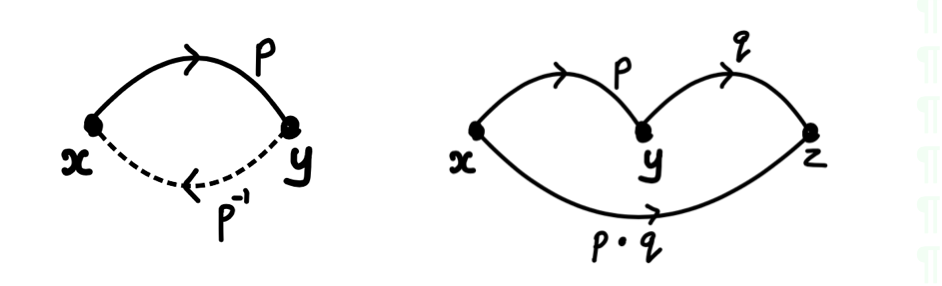
Symmetry: If is a path from to , we have an inverse path .
This can be seen by defining the inverse operation where we let . By path induction (J-rule) it is suffices to construct Define
Transitivity: We can concatenate paths and to produce a new path .
This can be seen by the concat operation: Denote . Again, by path induction it suffices to construct Define
Exercise 1: Show that concatenation is associative and satisfies and . In other words construct a term and and .
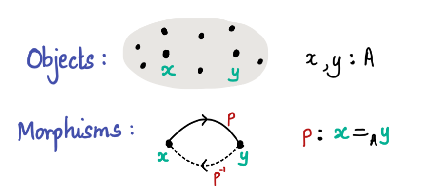
We can interpret types as groupoids!
A groupoid is category in which every morphism is invertible. In other words, every arrow in a groupoid can be inverted. The objects of the category are terms of a type and the morphisms between two terms are paths between and . Every morphism is invertible because of the existence of inverse paths. An explicit construction of this can be seen in this paper.
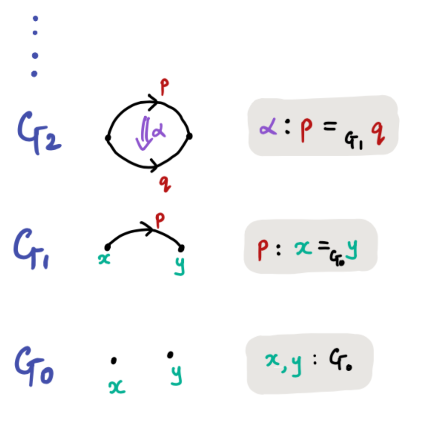
Towards an - groupoid structure of type theory
The first thing to observe is that is also a type and so it can be recognised as a groupoid. The morphisms in this groupoid are paths . There is no reason to stop here as we can also model the type as a groupoid. The arrows in this groupoid are now the higher dimensional paths . We can continue this process “up to infinity.”
As a result of the iterated application of J-rule, these “higher” types satisfy some nice coherence properties. These coherence properties allow us to the package this into an infinity groupoid.
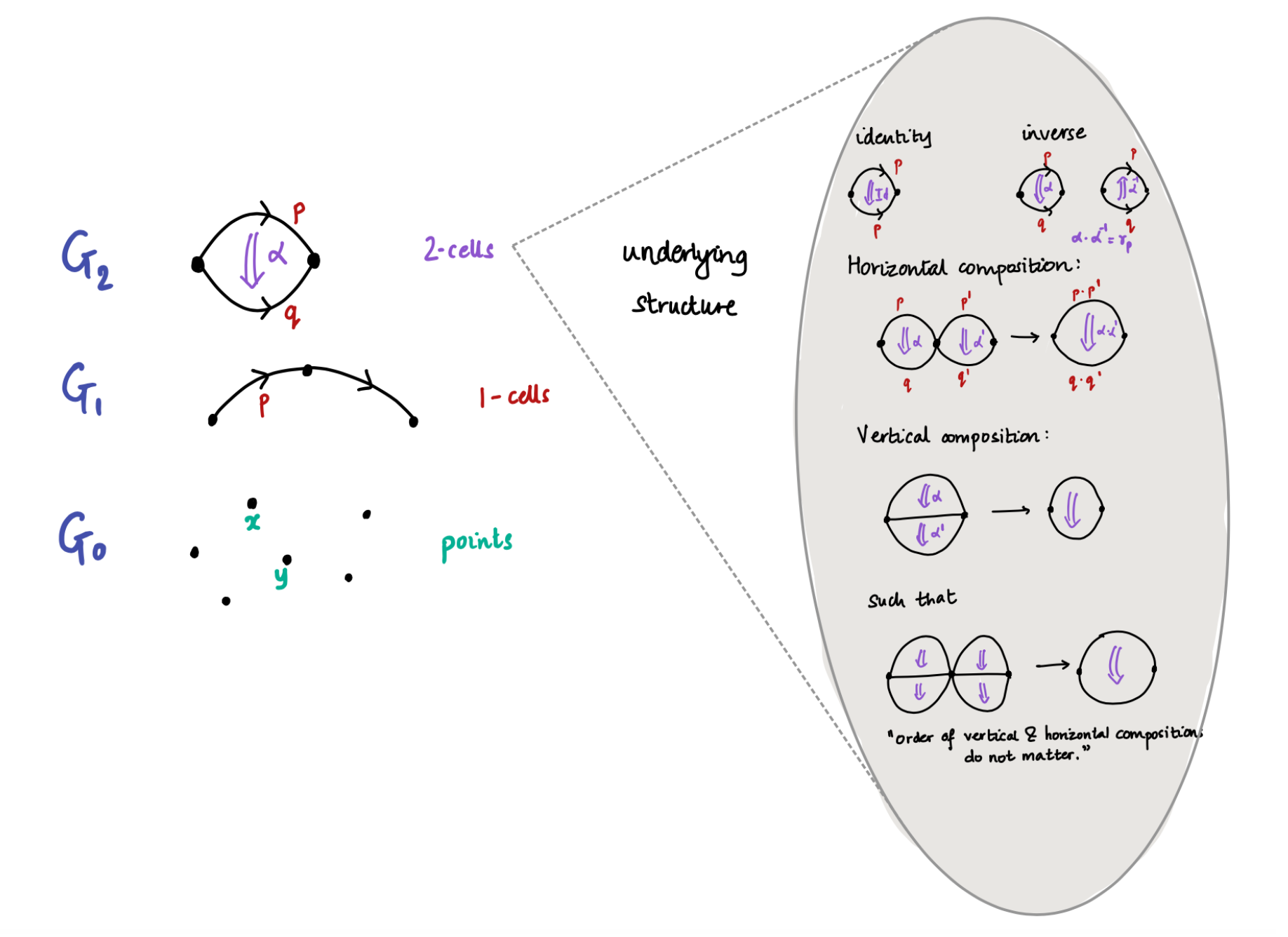
An infinity groupoid can be thought of as a family of sets for with additional structure: compositions, identity morphisms and inverse elements that satisfy unit, inverse and associativity laws “up to the next level.” Here is what “up to the next level” means in context of composition and associativity:
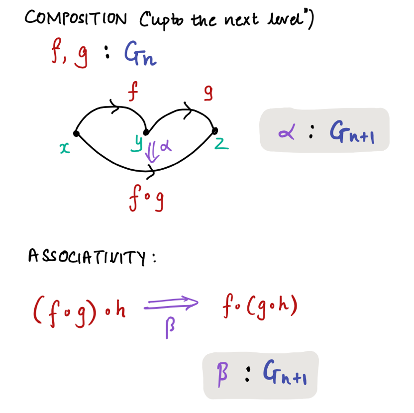
To summarise, is the set of points, is the set of 1-dimensional arrows between the points, is the set of 2-dimensional arrows (or the 2-cells) from any parallel pair of 1-dimensional arrows and so on.
Types can be packaged as infinity groupoids in the following sense:
The iterated application of J-rule for identity types gives us the coherence relations for free.
For example, in Exercise 1 we constructed a proof of associativity Here is a 2-cell and can be seen as term of . Similarly and are also 2-cells.
There are other models of type theory.6 Voevodsky observed that the groupoid and simplicial models of type theory satisfies a key property- called univalence. Univalence makes the relation between homotopy theory and type theory very clear. This is an extremely humble introduction to univalence, the true genuis of univalence can be seen here.
Univalence
In traditional set theory, any proof of should be equal. Following an example from Grayson, in classical set theory the following sentence is false. This is because, if is defined as a certain quotient of , their elements are different. If you’d ask any mathematician, though, they would say that there is really no problem in treating them as if they were the same, and in fact there is an isomorphism - actually more than one. Univalence is meant to implement this “as if” into a formal system. Before we state the axiom, we give a few definitions:
Let and be two functions. A homotopy from to is a function of type
A type is contractible when there is a point in . This means that there is some such that for every .7
The fiber of a function over a point is
The function is an equivalence of types if the fiber of is contractible over all points . We say is a term of type .
Example: A contractible type is equivalent to 1 (the type with one term ). This can be seen by the equivalence 1 sending for evry .
We are now ready to define the Univalence Axiom.
For any two types and ,
Equivalent types maybe identified.
Here, we haven’t specified in which type ‘=’ holds. There is a notion of types of types called universes and so we say more precisely, a universe is univalent if for all types .
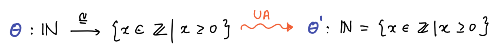
The power of the univalence axiom will be given in the next section and for now we content the reader with an example. The UA states that at element of can be thought of as providing a way to identify with .
In the presence of univalence, we no longer need to abuse notation to write
H-levels
Voevodsky observed that types can be stratified according to homotopy levels or h-levels. The h-level expresses the homotopy level of a type in following sense:
Contractible types
Types such that has h-level .
Note: In modern notation, h-level 0 is written as h-level -2 so that sets have homotopy level 0.
We now describe types of h-levels 1 and 2.
A type A is a proposition if any two terms of A are equal. In other words,
This is in accordance with our intuition that any two proofs of a proposition are equal.
By definition of h-levels, the h-level of propositions is 1.
A type A is a set if for all and all , we have . In other words, any two terms of a set are propositions. Formally,
Intuitively, we want a set to be a type that does not contain any higher homotopical information. This coincides with our intuition of sets- proofs of equality of sets are equal.
Example: is a set.
Non-Example: The type Group is not a set.
In the presence of UA, for any two groups and we have an equivalence, There may be multiple isomorphisms from to and so may have more than one element. So, the UA implies that may have more than one element which means that Group is NOT a set! But, the group isomorphisms type is a set and so under UA, the type is a set. This gives groups a h-level of 3. More generally, groupoids have h-level 3.
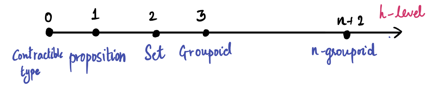
As you may guess, -groupoids have h-level . We end with a schematic view of the homotopy levels of types.
We have touched on different approaches and facets to identity in maths in general, and in type theory in particular. Pursuing a better understanding of it is not only the first step in the direction of a complete formalisation of mathematics, but a continuous source of inspiration.
1 … and can be made precise with the name of Equivalence Principle (EP). It intuitively states that two objects which are the same according to some notion of sameness share the same properties, if one only consider those that are relevant to that notion. A first attempt at relating this to univalence, introduced below, can be found here. ↩
2 In “Equality in hyperdoctrines and the comprehension schema as an adjoint functor” (1970) Lawvere shows that in the language of doctrines such properties fit into the description of a left adjoint: consider a functor (in loc.cit. the author assumes and to be cartesian closed for all in ). We can think of as the category of contexts or lists of sorts, and its morphisms as terms, then maps to each context the Lindenbaum-Tarski algebra of well-formed formulae in such context. Such a functor (called a doctrine) is said to be elementary if the image of the (parametrized) diagonal has a left adjoint satisfying Frobenius reciprocity and Beck-Chevalley. The unit of such an adjoint pair, for example, describes the reflexivity of this so called “equality”. ↩
3 Again, such interpretetation is merely a choice, for example in Identity and existence in intuitionistic logic (1979) Scott even questions the fact that should be the top element in the Boolean (in this case, Heyting) algebra, so that the one element should be equal to itself not with maximum “probability” or “certainty”, but only to the extent is exists in the system. ↩
4 ↩
5 This is from a very nice PhD course held by F. Dagnino and J. Emmenegger in Genova in the spring of 2022. ↩
6 Historically, there have been many definitions of -groupoids- globular sets, quasi categories (or Kan complexes) and topological categories. The model described above uses the globular sets defintion of -groupoids follwowing Berg and Garner.The Grothendieck homotopy hypothesis says
“Any topological space up to homotopy is essentially the same as an -groupoid”.
In the Kan complex definition of -groupoids, this hypothesis is true. There is a model of type theory in Kan complexes given by Veovodsky & Streicher (2006/2009). This allows us to interpret “types as topological spaces.” This was generalised to model structures in abstract homotopy theory by Awodey and Warren in 2006. ↩
7 Construct a type that checks if is contractible as follows: ↩
Re: Identity types in context
There is also the variant of the J-rule which is only valid up to a path, rather than judgmental equality; these are frequently found in cubical type theories for path types.