The n-Category Café

Tony goes swimming

Let’s warm up with a hypothetical scenario. Tony goes swimming once a week, on a variable day. What probability distribution on $\{Mon, Tue, Wed, Thu, Fri, Sat, Sun\}$ should we use to model his swimming habits?

If we have no information whatsoever, it’s got to be the uniform distribution $(1/7, \ldots, 1/7)$, purely by symmetry.

But now we might bring to bear our knowledge that swimming is a leisure activity, which makes it more likely to happen at weekends. Or perhaps Tony slips us a definite clue: he goes at weekends exactly as often as he goes on weekdays. Of course there are many distributions that satisfy this constraint, but again, symmetry compels us to choose

$$\Bigl( \frac{1}{10}, \frac{1}{10}, \frac{1}{10}, \frac{1}{10}, \frac{1}{10}, \frac{1}{4}, \frac{1}{4} \Bigr)$$

as the canonical answer.

Symmetry only gets us so far, though. What if Tony also tells us that the probability he goes on Friday is equal to the sum of Wednesday’s and Thursday’s probabilities? Any distribution

$$\Bigl( \frac{1}{4} - 2p, \frac{1}{4} - 2p, p, p, 2p, \frac{1}{4}, \frac{1}{4} \Bigr)$$

with $0 \leq p \leq 1/8$ satisfies the known constraints and the obvious symmetry requirements, and it’s not clear which of them should be regarded as “canonical”.

What are we doing?

What’s happening here is that we’re looking for the most uniform distribution possible, but except in simple cases, we can’t say what that means without some way of quantifying uniformity. So, let’s think about that. How uniform is a given probability measure on a space?

You may have guessed that this has something to do with entropy, and you’d be right. But I want to explain all this from the ground up, motivating everything from first principles, without invoking the E word. Also, if you guessed that what we’re going to end up with is a maximum entropy distribution, you’d only be half right. There are actually two key ideas here, and maximizing entropy is only one of them.

How spread out is a distribution?

The first key idea is to look for the most spread-out distribution possible on a space. I won’t say just yet what kind of “space” Emily and I worked with, but they include metric spaces, so you can keep that family of examples in mind.

Let’s consider this subset of $\mathbb{R}^2$:

It’s drawn here with an even shading, which corresponds to the uniform distribution — I mean, Lebesgue measure, normalized to give the space a total measure of $1$. But of course there are other probability measures on it, like this one with a single area of high concentration (shaded darker) —

— or this one, with two areas of high concentration —

Which one is the most spread out?

Of course, it depends what “spread out” means. It’s pretty clearly not the second one, where most of the mass is concentrated in the centre. But arguably the third is more spread out than the first, uniform, distribution: relative to the uniform distribution, some of the mass has been pushed out to the sides.

Or take this simpler example. Consider all probability measures on a line segment of length $1$, and let’s temporarily define the “spread” of a distribution on the line as the expected distance between a pair of points chosen randomly according to that distribution. An easy little calculation shows that with the uniform distribution, the average distance between points is $1/3$. But we can do better: if we put half the mass at one endpoint and half at the other, then the average distance between points is $1/2$. So the uniform distribution isn’t always the most spread out! (I don’t know which distribution is.)

This measure of spread isn’t actually the one we’ll use. What we’ll work with is not the distance between points, but the similarity between them.

Measuring spread

Formally, take a compact Hausdorff space $X$ and a “similarity kernel” $K$ on it, which means a continuous function $K \from X \times X \to \mathbb{R}^+$ such that $K(x, x) \gt 0$ for every point $x$. You can obtain such a space from a compact metric space by putting $K(x, y) = e^{-d(x, y)}$. That’s the most important family of examples.

Suppose we also have a probability measure $\mu$ on $X$. (Formally, “measure” means “Radon measure”.) We can quantify how ordinary or typical a point is with respect to the measure — in other words, how dark you’d colour it in pictures like the ones above. The typicality of $x \in X$ is

$$(K \mu)(x) = \int_X K(x, y) \,d\mu(y) \in \mathbb{R}^+.$$

It’s the expected similarity between $x$ and a random point. The higher it is, the more concentrated the measure is near $x$.

The mean typicality of a point in $X$ is

$$\int_X K\mu \,d\mu.$$

This is high if the measure is highly concentrated. For instance, if we’re dealing with a metric space then $K(x, y) = e^{-d(x, y)}$ always lies between $0$ and $1$, so the maximum possible value this can have is $1$, which is attained if and only if $\mu$ is concentrated at a single point — a Dirac delta. So, $\int K\mu \, d\mu$ quantifies the lack of spread. Hence

$$1 \Big/ \int_X K\mu \,d\mu$$

quantifies the spread of the measure $\mu$ across the space $X$.

But this is just one way of quantifying spread! More generally, instead of taking the arithmetic mean of the ordinariness (which is what $\int K\mu\,d\mu$ is), we can take any power mean. Then we end up with

$$1 \Big/ \Bigl(\int_X (K\mu)^t \,d\mu\Bigr)^{1/t}$$

as our measure of spread, for any real $t \neq 0$.

For reasons I won’t go into, it’s convenient to reparametrize with $t = q - 1$ and it’s sensible to restrict to $q \geq 0$. Simplifying, our formula becomes

$$D_q^K(\mu) = \Bigl( \int_X (K\mu)^{q - 1} \,d\mu \Bigr)^{1/(1 - q)}$$

($q \neq 1$). And although this formula doesn’t make sense when $q = 1$, taking limits as $q \to 1$ gives the righteous definition there:

$$D_1^K(\mu) = \exp\Bigl( - \int_X \log(K\mu)\,d\mu \Bigr).$$

If this sounds familiar, it might be because Christina Cobbold and I used $D_q^K(\mu)$ as measures of biological diversity. Here $X$ is to be thought of as a finite set of species, $K(x, y)$ indicates the degree of similarity between species (genetic, for instance), and $\mu$ is the relative abundance distribution of the species in some ecological community. High values of $D_q^K(\mu)$ indicate a highly diverse community. The parameter $q$ controls the relative emphasis placed on typical or atypical species: e.g. $q = 0$ gives atypical species as much importance as typical ones, while $q = \infty$ depends only on the most typical species of all.

In any case, Emily and I call $D_q^K(\mu)$ the diversity of $\mu$ of order $q$. Its logarithm,

$$H_q^K(\mu) = \log D_q^K(\mu),$$

is the entropy of $\mu$ of order $q$. In the special case where $X$ is finite and

$$K(x, y) = \begin{cases} 1 &\text{if } x = y \\ 0 &\text{if } x \neq y, \end{cases}$$

the entropy $H_q^K(\mu)$ is the Rényi entropy of order $q$, and in the even more special case where also $q = 1$, it’s the Shannon entropy.

For today it doesn’t matter whether we use the diversities $D_q^K(\mu)$ or the entropies $H_q^K(\mu)$, since all we’re interested in is maximizing them, and logarithm is an increasing function. So “diversity” and “entropy” mean essentially the same thing, and in this geometric context, they’re our formalization of the idea of “spread-outness”.

What’s the most spread-out distribution of them all?

Fix a space $X$ with a similarity kernel $K$, as above. You won’t lose much if you assume it’s a metric space $X$ with $K(x, y) = e^{-d(x, y)}$ if you like, but in any case, I’ll assume now that $K$ is symmetric. (The theorem I’m about to state needs this.)

Two questions:

• Which probability measure $\mu$ on $X$ maximizes the diversity $D_q^K(\mu)$?

• What is the value of the maximum diversity, $\sup_\mu D_q^K(\mu)$?

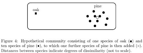
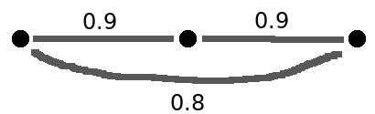
We’ve already observed that if we want to maximize diversity (“spread-outness”), the uniform distribution might not be best. We saw that for the line segment and the potato shapes. Another simple example is a three-point space consisting of two points very close together and the third far away. You wouldn’t want to use the uniform distribution, as that would put $2/3$ of the weight at one end and $1/3$ at the other. Something closer to $(1/4, 1/4, 1/2)$ would be more spread out.

So the answers to these questions aren’t going to be simple. But also, there’s an elephant in the room: both answers surely depend on $q$! After all, changing $q$ changes $D_q^K(\mu)$, and different values of $q$ sometimes have conflicting ideas about when one probability measure is more spread out than another. It can happen, for instance, that

$$D_0^K(\mu) \gt D_0^K(\nu) \qquad but \qquad D_1^K(\mu) \lt D_1^K(\nu)$$

for probability measures $\mu$ and $\nu$ on $X$.

However, Emily and I prove that it doesn’t actually matter! The answers to both questions are miraculously independent of $q$. That is:

• There is some probability measure $\mu$ that maximizes $D_q^K(\mu)$ for all $q \in [0, \infty]$ simultaneously.

• The maximum diversity $\sup_\mu D_q^K(\mu)$ is the same for all $q \in [0, \infty]$.

If this sounds familiar, it might be because Mark Meckes and I proved it in the case of a finite space $X$. Extending it to compact spaces turned out to be much harder than anticipated. For instance, part of the proof is to show that $D_q^K(\mu)$ is continuous in $\mu$, which in the finite case is pretty much a triviality, but in the compact case involves a partition of unity argument and takes up several pages of Emily’s and my paper.

What matters here is the first bullet point: there’s a best of all possible worlds, a probability measure $\mu$ on our space that unambiguously maximizes diversity (or entropy, or spread). Sometimes there’s more than one such measure. But in many examples, including many of the most interesting ones, there’s only one, so here I’ll casually refer to it as the most spread out measure on $X$.

Back to the line

The simplest nontrivial example is a line segment. What’s its most spread out measure?

Crucially, the answer depends on how long the line is. It’s a linear combination of 1-dimensional Lebesgue measure and a Dirac delta at each end, but the coefficients change with the length. I could write down the formula, which is simple enough, but that would distract from the main point:

As the length increases to $\infty$, the most spread out measure converges to normalized Lebesgue.

In other words, the Dirac measures at the end fade to nothing as we scale up.

The formal statement is this: if we write

$$K^t(x, y) = e^{-t|x - y|}$$

then for each real $t \gt 0$, the space $[0, L]$ with similarity kernel $K^t$ has a unique most spread out measure $\mu_t$, and in the weak${}^*$ topology on the space of probability measures, $\mu_t$ converges to the normalized Lebesgue measure on $[0, L]$ as $t \to \infty$.

Another term for “normalized Lebesgue measure” on the line is “uniform measure”. So in this example at least:

The uniform measure is the large-scale limit of the most spread out measure.

We’re going to take the lesson of this example and turn it into a general definition.

Defining the uniform measure

Here goes. Let $X$ be a compact metric space. Suppose that for $t \gg 0$, its rescaling $t X$ has a unique most spread out measure $\mu_t$, and that $\mu_t$ has a limit in the weak${}^*$ topology as $t \to \infty$. Then the uniform measure $\mu_X$ on $X$ is that limit:

$$\mu_X = \lim_{t \to \infty} \mu_t.$$

Conceptually, the difference between the “most spread out” measures $\mu_t$ and the uniform measure $\mu_X$ is that $\mu_t$ depends on the scale factor $t$ (as in the example of the line segment), but $\mu_X$ doesn’t. The uniform measure is independent of scale: $\mu_{u X} = \mu_X$ for all $u \gt 0$. That’s one of the properties that makes the uniform measure canonical.

In summary, the first key idea behind the definition of uniform measure is to take the most spread out (maximum entropy) distribution, and the second key idea is to then pass to the large-scale limit.

Recapturing the three examples

Back at the start of the post, I claimed that our notion of uniform measure captured three intuitive examples of the “canonical measure” on a space. Let’s check back in on them.

• Finite spaces.   For a finite metric space, the most spread out measure is not usually uniform, as we’ve seen. But as we scale up, it always converges to what’s usually called the uniform measure. In other words, what Emily and I call the uniform measure is, in this case, what everyone else calls the uniform measure.

  One way to think about this is as follows. In general, to get the uniform measure on a space $X$, we take the most spread out measure $\mu_t$ on $t X$ for each $t \gt 0$, then pass to the limit as $t \to \infty$ to get $\mu_X$. But for a finite space, we can do these two processes in the opposite order: first take the limit as $t \to \infty$ of $t X$, giving us a copy of $X$ where all distances between distinct points are $\infty$, and then take the most spread out measure on that space, which trivially is the one that gives equal measure to each point. This is just a story I tell myself: I know of no conceptual reason why interchanging the order of the processes should give the same result, and in any case the story only makes sense for finite $X$, since otherwise we escape the world of compact spaces. But perhaps it’s a helpful story.

• Homogeneous space.   Now take a compact metric space $X$ whose isometry group acts transitively on points. A version of the Haar measure theorem states that there’s a unique isometry-invariant probability measure $\mu$ on $X$. And it can be shown that the most spread out measure $\mu_t$ on $t X$ is just $\mu$. Taking the limit as $t \to \infty$, the uniform measure on $X$ is, therefore, also $\mu$.

  There’s a caveat here: the proof assumes that the metric space $X$ is of negative type, a classical condition that I don’t want to go into now. Many spaces are of negative type, including all subspaces of $\mathbb{R}^n$. But it would be nice to now whether the result also holds for spaces that aren’t of negative type.

  (And to be more careful than I really want to be in a blog post, it’s assumed here and in many other places that the space concerned is nonempty.)

• Subsets of $\mathbb{R}^n$.   In the case of a line segment, we saw that the uniform measure is the uniform measure in the usual sense (normalized Lebesgue). What about subsets of $\mathbb{R}^n$ in general?

  Let’s consider just those compact subsets $X$ of $\mathbb{R}^n$ that have nonzero measure. Then we can restrict Lebesgue measure to $X$ and normalize it to give $X$ a total measure of $1$. Is this canonical probability measure on $X$ the same as the uniform measure that Emily and I define?

  It is, and we prove it in our paper. A crucial role is played by a result of Mark Meckes: every compact subset of $\mathbb{R}^n$ has a unique most spread out measure. (The proof is Fourier-analytic.) But the point I want to emphasize is that unlike in the previous two examples, we have no idea how to describe $\mu_t$ for finite scale factors $t$!

  However, despite not knowing $\mu_t$ for finite $t$, we can describe the limit of $\mu_t$ as $t \to \infty$ — in other words, the uniform measure on $X$. And as promised, it’s precisely normalized Lebesgue.