Relational Universal Algebra with String Diagrams
Posted by Emily Riehl
.")
guest post by Phoebe Klett and Ralph Sarkis
This post continues the series from the Adjoint School of Applied Category Theory 2022. It is a summary of the main ideas introduced in this paper:
- Filippo Bonchi, Dusko Pavlovic and Pawel Sobocinski, Functorial Semantics for Relational Theories.
Just as category theory gives us a bird’s-eye view of all mathematical structures, universal algebra gives a bird’s-eye view of all algebraic structures (groups, rings, modules, etc.) While universal algebra leads to a beautiful theory with many general statements — it also enjoys a categorical formulation introduced in F.W. Lawvere’s thesis which inspired the aforementioned paper’s title — it does not deal with several common structures in mathematics like graphs, orders, categories and metric spaces. Relational universal algebra allows to cover these examples and more. In this post, we present this field of study using a diagrammatic syntax based on cartesian bicategories of relations.
Relational Algebras
We start by describing the classical (or non-categorical) view of relational theories because it should look more familiar to most people. The classical story starts with universal algebra, a field of mathematics that studies algebraic structures — like groups, rings, modules or lattices — from above. Instead of doing group theory, ring theory, etc., universal algebra formalizes what all these theories have in common to study algebraic theories all at once. An algebraic theory is the basic object of study in universal algebra, and it syntactically describes a kind of structure by asserting what types of operations can be done and the properties they satisfy. For instance, the theory of monoids contains
- a symbol that takes two inputs and a symbol that takes no inputs, and
- axioms that stipulate how these symbols can be manipulated.
While theories embody the syntax wielded by an algebra professor on the blackboard, students understand the meaning of these obscure symbols using models. A model for a theory is an interpretation of the symbols that instantiates the structure described, e.g., models of the theory of monoids are monoids.
The limit of universal algebra is that the structures have to be sets equipped with functions of type . This does not cover things that are not intuitively algebraic, e.g., graphs, orders, metric spaces. Relational algebraic theories can cover all these examples as well as all algebraic theories.
Let us go quickly through the definitions before giving more insight with examples.
Definition: A relational signature is a set of symbols, each with an arity and coarity in . We write for a symbol of arity and coarity belonging to .
Definition: A model of is a set , called the carrier, equipped with a relation for every . A morphism of models is a function between the carriers that preserves all relations in the signature, i.e., satisfying
Examples:
- Models of the empty signature are simply sets, and their morphisms are functions with no constraints.
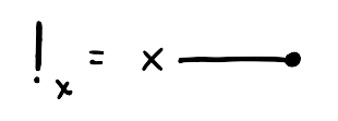
- Models of are sets equipped with a predicate, i.e., a subset of . For two predicates and , a function preserves the predicate iff , or, written differently, .
- Models of are sets equipped with a binary relation, i.e., a subset of . Given binary relations and on and respectively, a function is a morphism iff .
To obtain more interesting objects, we need to impose axioms on the relations in the signature, e.g.,
- a poset is a set with a binary relation that is reflexive, transitive and antisymmetric
- an undirected graph (with loops) is a set with a binary relation that is symmetric
- a magma is a set with a relation between and that is a function, namely, each element of is related to exactly one element in .
In universal algebra, axioms are imposed by equations between terms constructed using the symbols of the theory. The theory of monoids, for instance, contains the following three equations
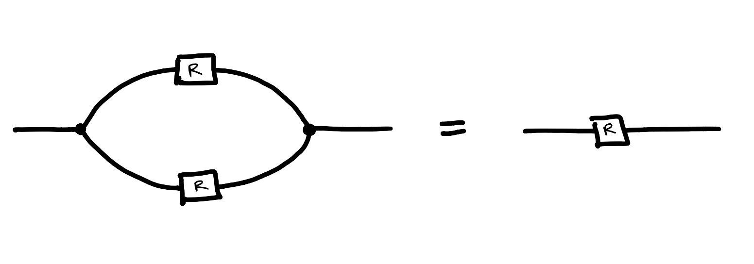
which imply that, in every model, the monoid operation is associative and has as its neutral element (on the left and right). It is not hard to design something similar for posets. The structure consists of a binary relation , and the axioms are (where is the identity or diagonal relation and denotes composition of relations)
For now, you can believe us that these assert reflexivity, transitivity, and antisymmetry respectively.
The terms , , , and , were constructed using only the syntax that is part of the theory of monoids, while the axioms in the theory of posets rely on the identity relation and the composition and intersection of relations in addition to the symbols in the signature. Moreover, the axioms are stated as inequations rather than equations.
Cartesian Bicategory of Relations
In this section, we describe a diagrammatic syntax that will be used to specify axioms of a theory, and in particular, to construct complex relations out of symbols in the signature. This syntax comes from the structure of a cartesian bicategory of relation. We will introduce this notion by looking at one particular instance of it: the category of sets and relations.
The objects of are sets, and a morphism in is a subset of that we call a relation from to . The composition of two relations and is defined by and the identity relation is .
The categorical product in is the disjoint union of sets (it is also the coproduct), so the Cartesian product of sets does not satisfy the usual universal property. (For those who already know about functorial semantics of algebraic theories, this explains why the naive attempt to describe relational algebras as -valued cartesian functors fails.) However, equipped with the Cartesian product is a cartesian bicategory of relations, namely, it is poset-enriched, symmetric monoidal, and it is a hypergraph category where convolution is idempotent. Let us unroll this.
is enriched in the category of posets and order-preserving maps. Explicitly, we can see the Hom-set as the powerset , then (set inclusion) is a partial order, and one can check for any and , .
equipped with the Cartesian product of sets is a symmetric monoidal category. Indeed, the Cartesian product of sets is associative (up to isomorphisms), and the singleton is the unit, i.e., for any set , . For any two relations and , we define One can check that the interchange identity holds and the Cartesian product preserves the order, i.e., for any and , For any sets and , the braiding is the relation
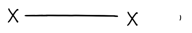
We can summarize the last paragraph by saying how we can manipulate relations with string diagrams. For any set , we draw the identity relation on as a single wire
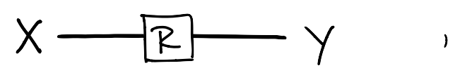
we draw a relation as a box
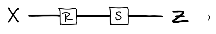
we draw the composition of two relations and as the sequential composition of boxes
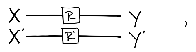
we draw the product of relations and as parallel composition of boxes
and, finally we draw the braidings as wires crossing
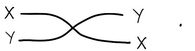
This two dimensional syntax is that it is topologically sound. This means you can manipulate a diagram as you if you were moving actual wires connected to boxes on a table, and if you do not break/cut any connection and leave the boundary (the input and output wires) untouched, then the diagram you started with and the diagram you end up with represent the same relation. Here is an example of two diagrammatic representations of the same relation.
In addition, with a bit of visual imagination, one can figure out the relation represented by a diagram without translating to the classical syntax. We abstain from explaining this process here, but we can recommend these wonderful videos that introduce a syntax very similar to ours.
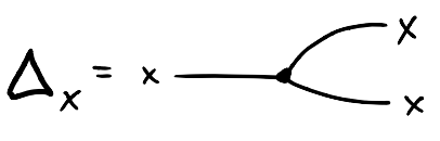
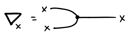
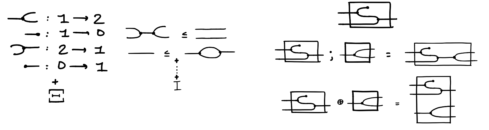
equipped with is a hypergraph category because every set can be coherently equipped with a special commutative Frobenius algebra structure. Explicitly, given a set , there are four relations , , and depicted below that satisfy a bunch of equations listed below.
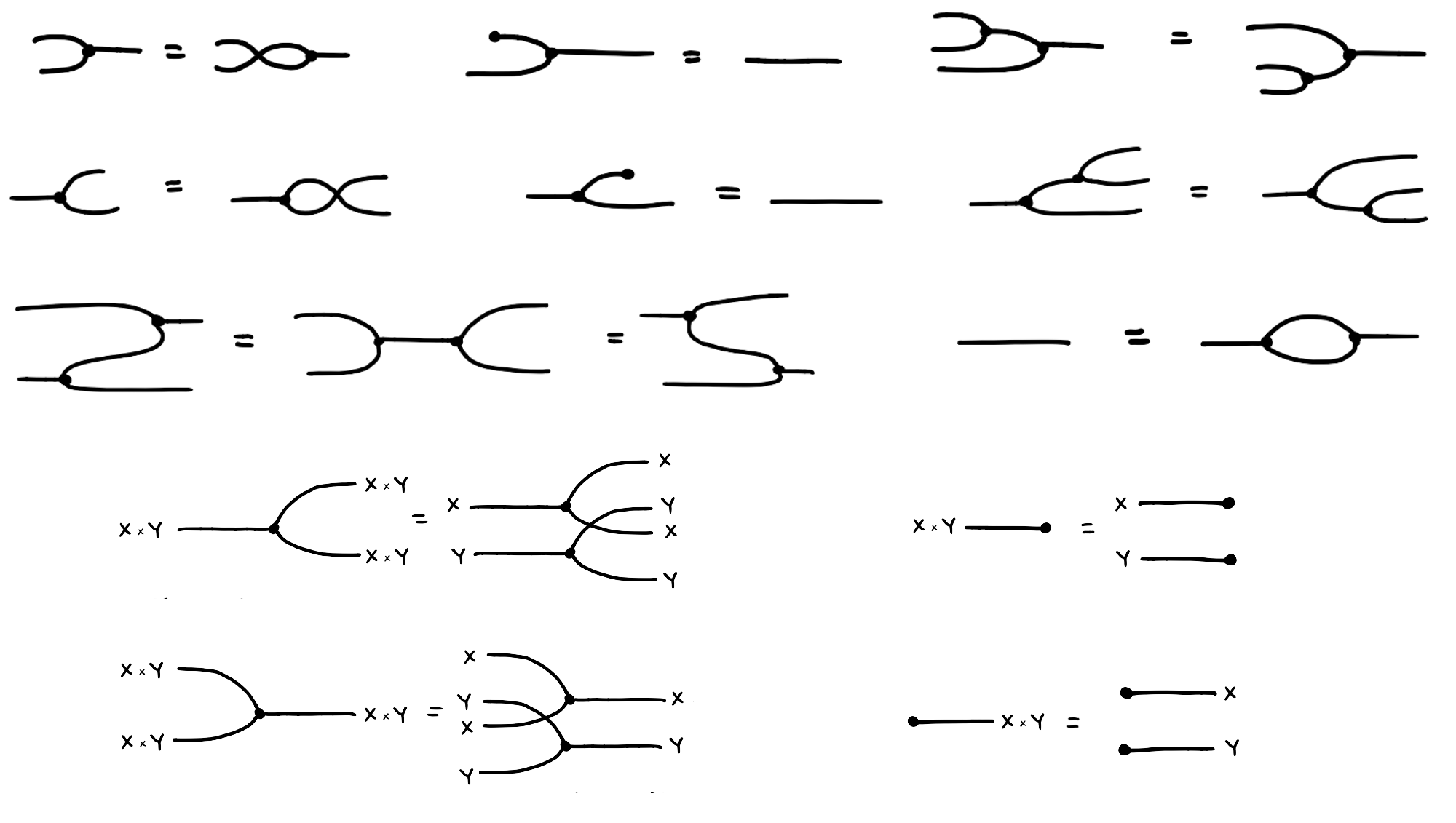
For our purposes, all of this is simply additional syntax that we can use to construct relations. These equations mean that whenever you see the left hand side of an equation within a bigger diagram, you can replace it with the right hand side without altering the meaning of the bigger diagram.
Finally, convolution in is idempotent. Given two relations , the convolution of and is the relation drawn as
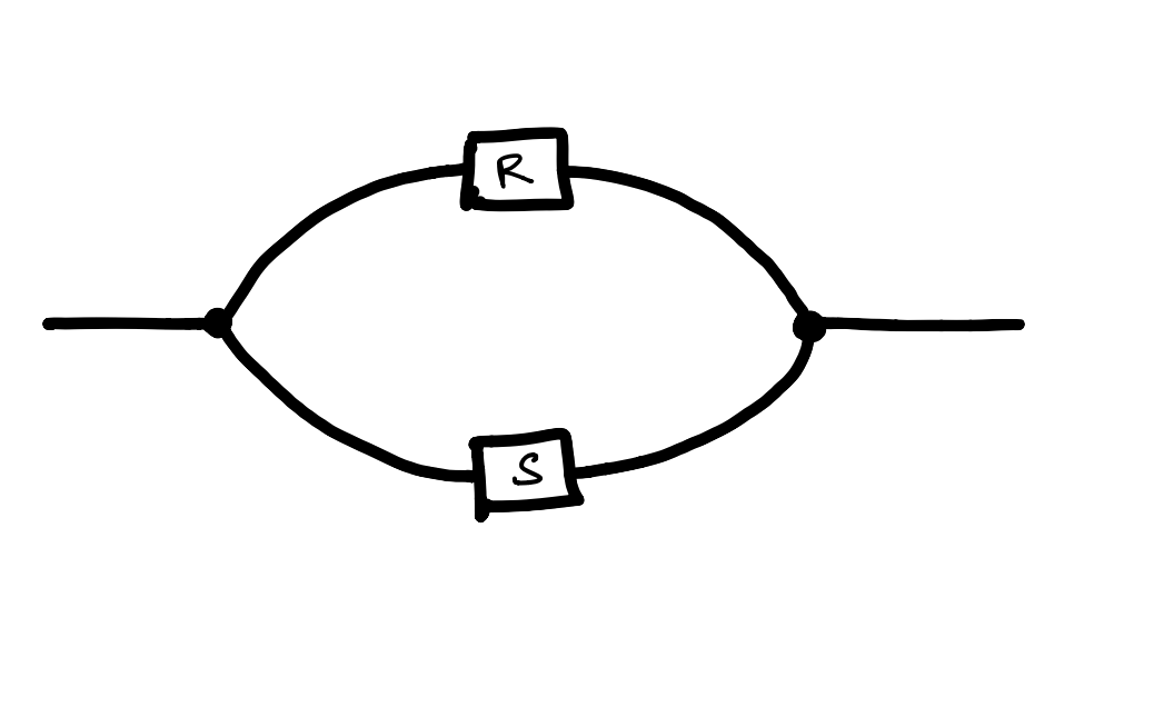
Puzzle: What is the convolution of and ?
The solution is given later in the post, but for now, it is important to note that for any relation , the convolution of with itself is equal to , that is, convolution is idempotent.
Recall that we introduced the diagrammatic syntax of cartesian bicategories of relations because we wanted a language to express axioms of a theory of relational algebras. The following section is devoted to such theories.
Frobenius Theories
Now that we’ve been introduced to the ideas of universal algebra and the syntax of cartesian bicategories of relations, we can start to talk about theories of a categorical flavor, theories in functorial semantics, and specifically Frobenius theories as introduced by the authors of the paper. The definition of a theory in this case looks very similar to that of universal algebra.
Given a relational signature , a Frobenius -term is a string diagram constructed with the generators in and the syntax of cartesian bicategories of relations. This construction of terms will allow us to express and impose axioms on more complex terms, as we lacked in the previously discussed theories.
A Frobenius theory is a pair consisting of a relational signature and a set of inequations , i.e., pairs where and are Frobenius -terms. Note that inequationas are at least as powerful as equations since, in the interpretation outlined below, having would be equivalent to having and . We often call theories with inequations lax theories, as we’ve relaxed the equality into an inequality.
Let’s see an example. The Frobenius theory of posets can be described with one generating relation and 3 inequations.
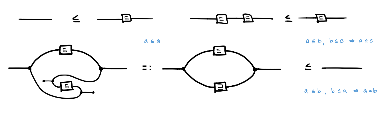
Translating between the string diagrams and axioms (in blue) is achieved using models of the theory, which will be discussed shortly.
Given a theory , we can generate a Frobenius prop or “frop” for short. A prop is a strict symmetric monoidal category, where the objects are the natural numbers and the monoidal product is addition. Arrows are string diagrams with input wires and output wires.
Just as we can generate a vector space from a set of basis vectors, we can generate a prop from a theory. Given the (co)monoid structure of cartesian bicategories of relations, along with any generating relations of the theory, we can freely construct terms or arrows in our frop using sequential and parallel composition.
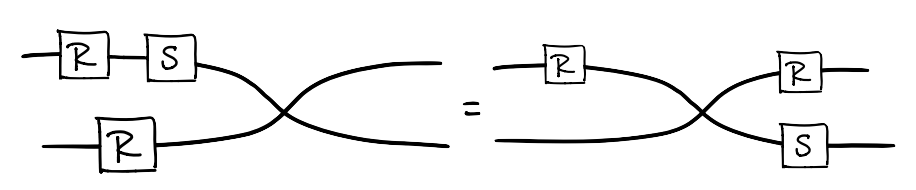
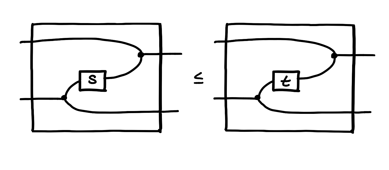
Arrows in are Frobenius -terms modulo laws of cartesian bicategories of relations, modulo smallest congruence with respect to containing equations . This means for a pair we can swap out these terms in our arrows as shown below.
Models of a Frobenius Theory
Earlier we discussed models of a theory as instances of the thing we care about. (I.e. if we’re studying the theory of groups, a model in that case is a choice of group.) Functorial semantics is a categorical perspective of what it means to be a model. Namely, models of Frobenius theories are functors of a specific type.
Explicitly, a model for a Frobenius theory is a functor from , the frop generated by , to a cartesian bicategory of relations such that preserves the structure of cartesian bicategories of relations. For intuition, we’ll use in this post.
To continue with the analogy of vector spaces, to understand how a linear transformation behaves we only need to consider how it acts on the basis vectors. In our case, in order to understand how our model behaves we only need to consider how it acts on the generating relations. And in order to interpret our inequations in the new setting of we simply apply our model. We illustrate the example of posets below.
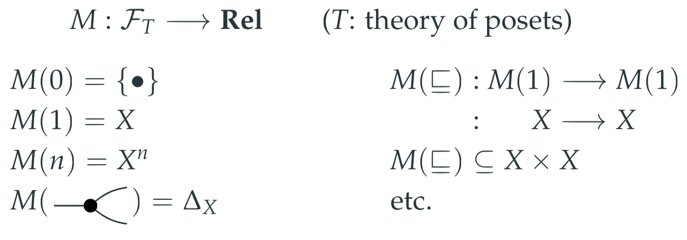
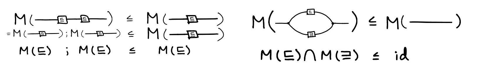
Note that we used the solution of the puzzle above: the convolution of and is their intersection.
What about morphisms of models? To understand the category of models, we need to know what arrows in that space look like. Morphisms of models are natural transformations, and in the Frobenius case, a morphism of models is a monoidal lax natural transformation.
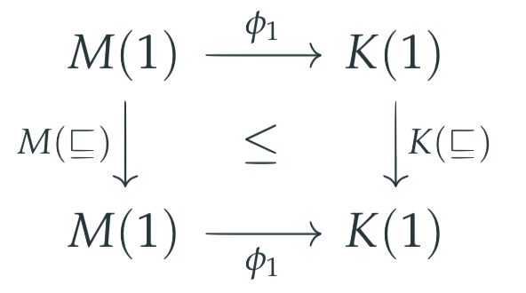
In particular, given ,
is the data
But since we know (in the Frobenius case) that this natural transformation is monoidal, we can conclude that it’s determined by .
We also know that for all the diagram below laxly commutes.
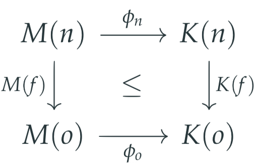
We consider the interesting cases when is the (co)monoidal terms and any generating terms in the signature.
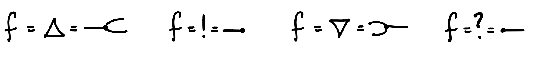
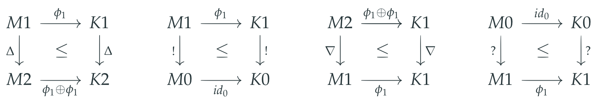
Inequations for and hold for any relation , but inequations for and hold if and only if the relation is a .
When is the generating relation in signature of posets, we arrive at the function being order preserving.
In general for any theory, a morphism in the category of models is a function preserving the relations. And this is the same as we had in the classical view. In cases where the classical models of universal algebra are equally expressive as the models of functorial semantics, their models are isomorphic. This is true for example in the case of Monoids.
Examples
Let’s see a few more examples.
What is the category of models for the empty Frobenius theory
?
This is just the category of sets and functions. models are uniquely determined by the object , which is just a set, and as we saw before, morphisms of models are functions.
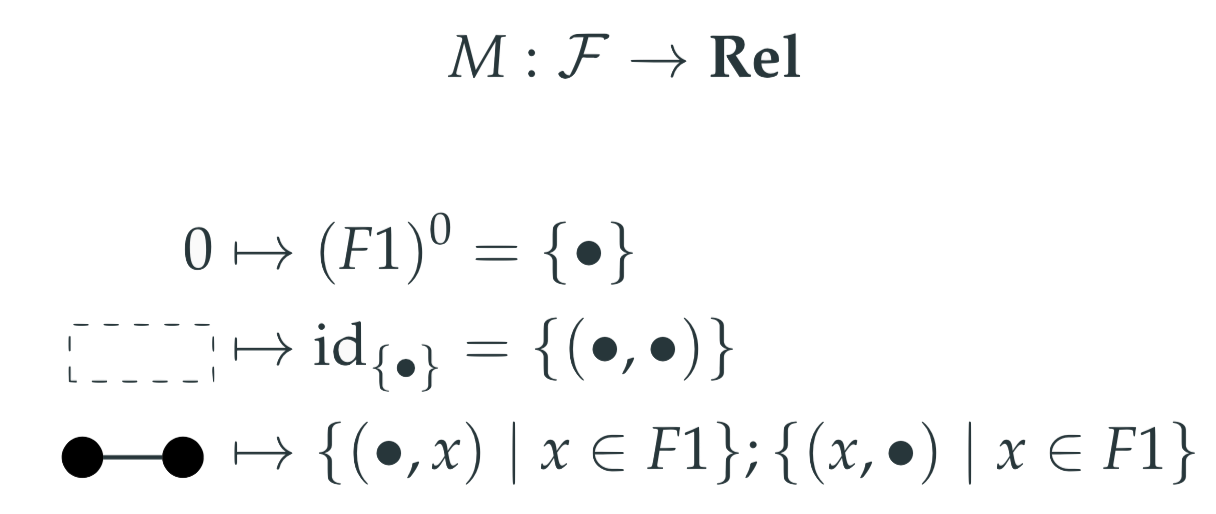
What about if we add the following inequation to ?
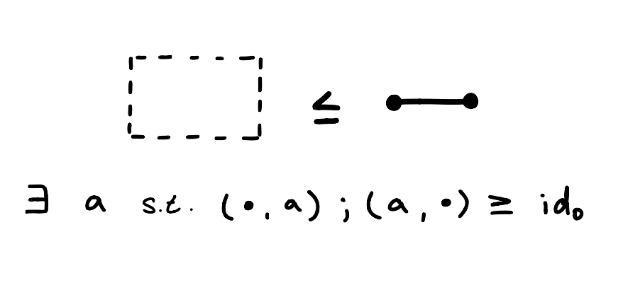
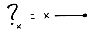
How do we even interpret this inequation? The right hand side can be decomposed into the composition of the unit and the counit, and relationally can be interpreted as “there exists an object such that it’s related to the (co)unit”. This is true for any object , so this inequation is just asking us to have an element in our set, or for our set to be nonempty.
Models are sets that contain at least one element.
Let’s take semigroups, roughly groups where we forget about identities and inverses. We define the signature and equations as below.
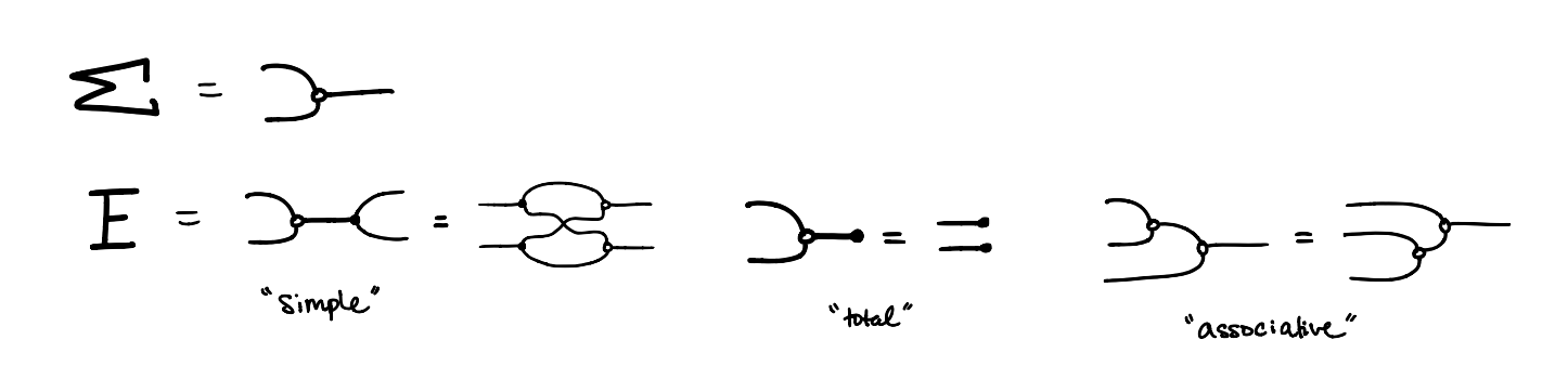
How should we interpret these equations?
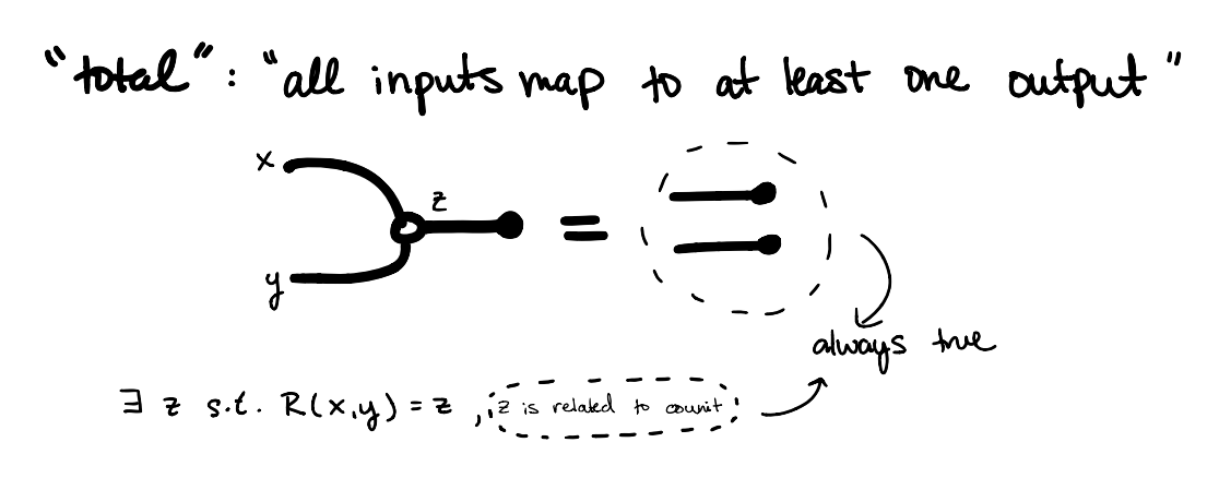
Consider the inequation called “total”. Intuitively, total asks that all inputs map to at least one output. We can see this in the diagram by noting that both the right hand side and the right most term on the left hand side are always true, leaving only the first term on the left side, which simply quantifies the output of any input . or “there exists some such that ”.
If we add the following equation, we get regular semigroups, or semigroups where for any , there exists such that .
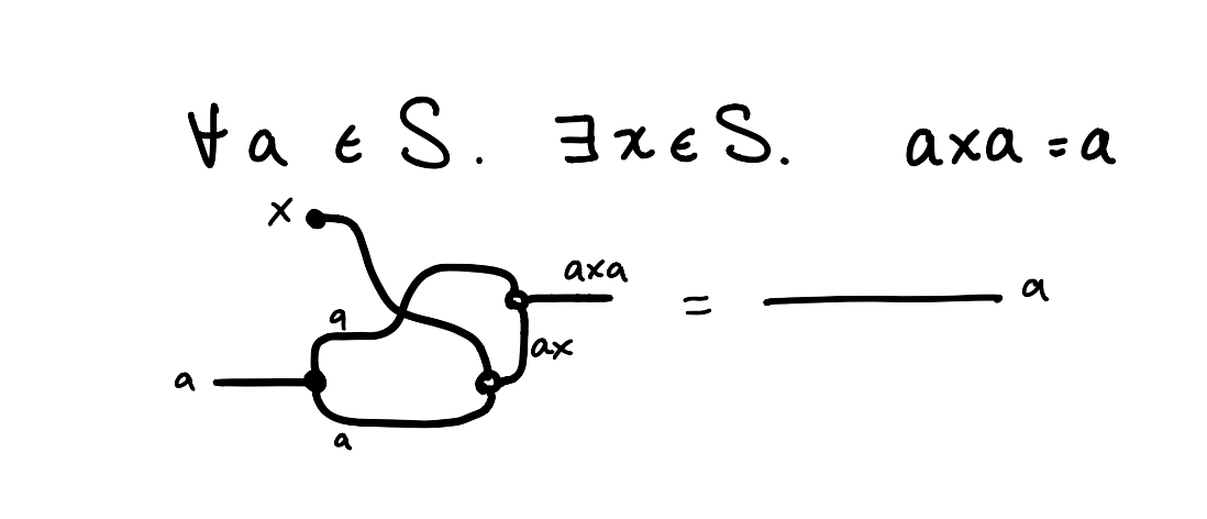
If you picture and coming in along the strings here, being copied/multiplied at the nodes, you can follow along to this conclusion.
The category of models and model morphisms is the category of regular semigroups and semigroup homomorphisms.
Re: Relational Universal Algebra with String Diagrams
Nice!
It’s not at all important, but I’m don’t remember hearing the word “inequation” — the people I know seem to say “inequality”. So when you said “inequation” at first I thought you meant . I was relieved to see you meant (or ).