Skip to the Main Content

Note:These pages make extensive use of the latest XHTML and CSS Standards. They ought to look great in any standards-compliant modern browser. Unfortunately, they will probably look horrible in older browsers, like Netscape 4.x and IE 4.x. Moreover, many posts use MathML, which is, currently only supported in Mozilla. My best suggestion (and you will thank me when surfing an ever-increasing number of sites on the web which have been crafted to use the new standards) is to upgrade to the latest version of your browser. If that's not possible, consider moving to the Standards-compliant and open-source Mozilla browser.

March 13, 2024

Counting Points on Elliptic Curves (Part 2)

Posted by John Baez

Last time I explained three ways that good curves can go bad. We start with an equation like

y 2=P(x) y^2 = P(x)

where PP is a cubic with integer coefficients. This may define a perfectly nice smooth curve over the complex numbers — called an ‘elliptic curve’ — and yet when we look at its solutions in finite fields, the resulting curves over those finite fields may fail to be smooth. And they can do it in three ways.

Let’s look at examples.

The good

In The Riemann Hypothesis (Part 2) we looked at a case of good reduction: an elliptic curve that stays smooth when we work modulo some prime. This curve wasn’t in the standard form I’ve been talking about recently. Instead, it looked like this:

y 2+y=x 3+x y^2 + y = x^3 + x

But that’s okay, it’s still an elliptic curve. It turns out to have good reduction at the prime p=2p=2. And this manifests itself when we count points on this curve over the fields 𝔽 q\mathbb{F}_q where q=p nq = p^n. To count these points we just count solutions of the above equation in 𝔽 q\mathbb{F}_q and add 11 for the ‘point at infinity’. We get a number I’ll call |E(𝔽 q)||E(\mathbb{F}_q)|, where EE is our elliptic curve:

n q=2 n |E(𝔽 q)| 1 2 5 2 4 5 3 8 5 4 16 25 5 32 25 6 64 65 7 128 145 8 256 225 9 512 545 10 1024 1025 11 2048 1985 12 4096 4225 \begin{array}{rrr} n & q = 2^n \! & \; |E(\mathbb{F}_q)|\\ 1 & 2 & 5 \\ 2 & 4 & 5 \\ 3 & 8 & 5 \\ 4 & 16 & 25 \\ 5 & 32 & 25 \\ 6 & 64 & 65 \\ 7 & 128 & 145 \\ 8 & 256 & 225 \\ 9 & 512 & 545 \\ 10 & 1024 & 1025 \\ 11 & 2048 & 1985 \\ 12 & 4096 & 4225 \\ \end{array}

You can see a lot of patterns here: for example, the number of points is 2 n2^n plus a slower-growing correction. We thought about that correction, and ultimately guessed that

|E(𝔽 q)|=2 n(1+i) n(1i) n+1 |E(\mathbb{F}_q)| = 2^n - (-1 + i)^n - (-1 - i)^n + 1

In fact this sort of formula is typical for primes of good reduction:

Theorem 1: Hasse’s Theorem on Elliptic Curves. Given a cubic equation with integer coefficients in two variables that defines an elliptic curve EE with good reduction at pp, we have

|E(𝔽 q)|=p nα nα¯ n+1 |E(\mathbb{F}_q)| = p^n - \alpha^n - \overline{\alpha}^n +1

where α\alpha \in \mathbb{C} has |α|=p|\alpha| = \sqrt{p}.

The Weil Conjectures, now theorems, say how this formula can be vastly generalized. Ultimately this led Grothendieck and others to think about ‘motives’. I said much more about this here. But now let’s move on to the other cases!

The bad: additive reduction

One kind of ‘bad reduction’ happens when our elliptic curve gets a cusp over 𝔽 p\mathbb{F}_p. To see this pattern it’s easiest to do a cubic curve that’s not even elliptic in the first place. Let’s try this one:

y 2=x 3 y^2 = x^3

This is not an elliptic curve because it already fails to be smooth over \mathbb{C}. It has a cusp, visible already in the real solutions:

The cusp is the pointy thing. So we should expect that working over some primes pp this curve will still have a cusp… and maybe this will affect the count of points in 𝔽 q\mathbb{F}_q when q=p nq = p^n.

It does! Let’s take the prime 22 again:

n q=2 n |C(𝔽 q)| 1 2 3 2 4 5 3 8 9 4 16 17 5 32 33 6 64 65 7 128 129 8 256 257 9 512 513 10 1024 1025 \begin{array}{rrr} n & q = 2^n \! & \; |C(\mathbb{F}_q)|\\ 1 & 2 & 3 \\ 2 & 4 & 5 \\ 3 & 8 & 9 \\ 4 & 16 & 17 \\ 5 & 32 & 33 \\ 6 & 64 & 65 \\ 7 & 128 & 129 \\ 8 & 256 & 257 \\ 9 & 512 & 513 \\ 10 & 1024 & 1025 \\ \end{array}

You can see the pattern is very different, and it’s much simpler. We just get 2 n+12^n +1.

When an elliptic curve has bad reduction at a prime pp because it gets a cusp, we say it has additive reduction. Here’s what happens then:

Theorem 2. Given a cubic equation with integer coefficients in two variables that defines an elliptic curve EE with additive reduction at pp, we have

|E(𝔽 q)|=p n+1 |E(\mathbb{F}_{q})| = p^n + 1

There’s a reason for this. You’ll notice that p n+1=q+1p^n + 1 = q + 1 is just the number of points in the projective line over 𝔽 q\mathbb{F}_q. And indeed, it turns out that in this case the curve E(𝔽 q)E(\mathbb{F}_{q}) is just a projective line that’s been mapped into the projective plane in a way that’s one-to-one, but fails to be smooth at the cusp.

Now what’s with this term ‘additive reduction’? Well, you may have heard that an elliptic curve is an algebraic group. There’s a way to add or subtract points on the curve —- a sneaky geometric construction that involves drawing lines between these points:

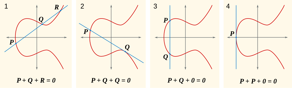
This still works over finite fields. So in cases of good reduction, E(𝔽 q)E(\mathbb{F}_{q}) is an algebraic group.

All this still works when our curve has a cusp — if you remove the cusp. When you remove the cusp you still get an algebraic group. In particular, the identity of this group is the point at infinity, and we haven’t removed that. And remember, in this case E(𝔽 q)E(\mathbb{F}_{q}) is secretly a projective line except for one non-smooth point at the cusp. So when you remove the cusp you get an ordinary affine line. So it’s not surprising that as an algebraic group, what’s left is isomorphic to the additive group of 𝔽 q\mathbb{F}_q.

That’s why this case is called ‘additive reduction’.

The ugly: split multiplicative reduction

Now for another kind of bad reduction. We say an elliptic curve has multiplicative reduction at the prime pp if gives a curve 𝔽 p\mathbb{F}_p that has a node. A node is a point with two different tangent lines — it’s easy to visualize in the real case:

But over a finite field, when you try to compute the slopes of the lines tangent to the node, they may or may not be defined over that field! The reason is that you need to solve some polynomial equations, and finite fields aren’t algebraically complete. If the tangent lines are defined over 𝔽 p\mathbb{F}_p we say our elliptic curve has split multiplicative reduction, otherwise we say it has nonsplit multiplicative reduction.

Here’s an elliptic curve with split multiplicative reduction over 𝔽 5\mathbb{F}_5:

y 2=x 3x 2+5 y^2 = x^3 - x^2 + 5

I only know this because someone says so — but I know how to check it, and someday I will. For now let’s just count the number of points over 𝔽 q\mathbb{F}_q when q=5 nq = 5^n. I have some cheap software that gets really slow when our prime gets as big as 55, so this table will be pretty small:

n q=5 n |E(𝔽 q)| 1 5 5 2 25 25 3 125 125 4 625 625 \begin{array}{rrr} n & q = 5^n \! & \; |E(\mathbb{F}_q)|\\ 1 & 5 & 5 \\ 2 & 25 & 25 \\ 3 & 125 & 125 \\ 4 & 625 & 625 \\ \end{array}

Luckily the pattern is obvious! And that’s how this case always works:

Theorem 3. Given a cubic equation with integer coefficients in two variables that defines an elliptic curve EE with split multiplicative reduction at pp, we have

|E(𝔽 q)|=p n |E(\mathbb{F}_{q})| = p^n

Again there’s a reason. Now p np^n is one less than the number of points in the projective line over 𝔽 q\mathbb{F}_q. The reason is that in this case, we get the curve E(𝔽 q)E(\mathbb{F}_{q}) by mapping the projective line into the projective plane in a way that crosses itself at the node. In other words this map is one-to-one except at the node, where it’s two-to-one.

We can can also get an algebraic group out of E(𝔽 q)E(\mathbb{F}_{q}) if we remove the node. When we do that, we’re left with projective line with two points removed — or an affine line with one point removed. So it’s not surprising that as an algebraic group, we get the multiplicative group of 𝔽 q\mathbb{F}_q, namely

𝔽 q ×=𝔽 q{0} \mathbb{F}_q^\times = \mathbb{F}_q - \{0\}

with multiplication as its group operation.

That’s why this case is called ‘multiplicative’.

The weird: nonsplit multiplicative reduction

Here’s a curve with non-split multiplicative reduction at p=3p = 3:

y 2=x 3x 2 y^2 = x^3 - x^2

And here is the count of points over 𝔽 q\mathbb{F}_q where q=3 nq = 3^n:

n q=3 n |E(𝔽 q)| 1 3 5 2 9 9 3 27 29 4 81 81 5 243 245 6 729 729 7 2187 2189 \begin{array}{rrr} n & q = 3^n \! & \; |E(\mathbb{F}_q)|\\ 1 & 3 & 5 \\ 2 & 9 & 9 \\ 3 & 27 & 29 \\ 4 & 81 & 81 \\ 5 & 243 & 245 \\ 6 & 729 & 729 \\ 7 & 2187 & 2189 \end{array}

The pattern is again quite evident, and this case always works this way:

Theorem 4. Given a cubic equation with integer coefficients in two variables that defines an elliptic curve EE with nonsplit multiplicative reduction at pp, we have

|E(𝔽 q)|=p n |E(\mathbb{F}_{q})| = p^n

when nn is even and

|E(𝔽 q)|=p n+2 |E(\mathbb{F}_{q})| = p^n + 2

when nn is odd.

We can play the same game as before and remove the node from E(𝔽 q)E(\mathbb{F}_q). The result is again an algebraic group over 𝔽 q\mathbb{F}_q. When nn is even everything works just as in the split case: this algebraic group has q1q - 1 points, it’s an affine line with one point removed, and it’s the multiplicative group 𝔽 q ×\mathbb{F}_q^\times.

But when nn is odd things get weird! Now our algebraic group has q+1q + 1 points. This is just as many points as the projective line over 𝔽 1\mathbb{F}_1. But there’s no way to make the projective line into an algebraic group! So what are we getting?

Well, we’re getting some weird algebraic group that only exists thanks to the fact that 𝔽 q\mathbb{F}_q is not algebraically closed!

1-dimensional connected algebraic groups

Indeed there are some theorems that go like this:

Theorem 5. Over an algebraically closed field kk the only connected 1-dimensional algebraic groups are:

  • elliptic curves (which are projective algebraic groups)
  • the additive group of kk (which is an affine algebraic group)
  • the multiplicative group k ×k^\times (which is an affine algebraic group).

Theorem 6. Over 𝔽 q\mathbb{F}_q the only connected 1-dimensional algebraic groups are:

  • elliptic curves (which are projective algebraic groups)
  • the additive group of kk (which is an affine algebraic group)
  • the multiplicative group k ×k^\times (which is an affine algebraic group).
  • one more connected 1-dimensional affine algebraic group.

Note that all these groups are abelian! The last one, the mysterious one, is what shows up when we study elliptic curves with non-split multiplicative reduction.

For more detail on everything I’ve said, and much more about that mysterious connected 1-dimensional affine algebraic group, go here:

Reid Barton pointed me to this article. It’s really great, and the only reason for writing mine is that I feel this subject deserves a more elementary introduction.

But before I quit, I want to look at an example of this mysterious connected 1-dimensional affine algebraic group. I want to hold this exotic entity in my hand and gaze at it.

Youcis says it’s the kernel KK of some homomorphism from the multiplicative group 𝔽 q 2 ×\mathbb{F}^\times_{q^2} onto the multiplicative group 𝔽 q ×\mathbb{F}^\times_q. In other words, it fits into an exact sequence

1K𝔽 q 2 ×f𝔽 q ×1 1 \longrightarrow K \longrightarrow \mathbb{F}^\times_{q^2} \stackrel{f}{\longrightarrow} \mathbb{F}^\times_q \longrightarrow 1

Let’s do a couple sanity checks. First of all, 𝔽 q ×\mathbb{F}^\times_q is a 1-dimensional algebraic group over 𝔽 q\mathbb{F}_q, while 𝔽 q 2 ×\mathbb{F}^\times_{q^2} is 2-dimensional. So, just counting dimensions naively, we expect that KK is 1-dimensonal.

We can also count points: our exact sequence implies

|𝔽 q 2 ×|=|K||𝔽 q ×| |\mathbb{F}^\times_{q^2}| = |K| \cdot | \mathbb{F}^\times_q |

or in other words

(q 21)=|K|(q1) (q^2 - 1) = |K| \cdot (q-1)

so

|K|=q 21q1=q+1 |K| = \frac{q^2 - 1}{q - 1} = q + 1

as we want. And if you’ve ever read my stuff on qq-arithmetic, this should bring back fond memories.

But what is this group like?

For that, we need to understand the map ff here a bit better:

1K𝔽 q 2 ×f𝔽 q ×1 1 \longrightarrow K \longrightarrow \mathbb{F}^\times_{q^2} \stackrel{f}{\longrightarrow} \mathbb{F}^\times_q \longrightarrow 1

The field 𝔽 q 2\mathbb{F}_{q^2} is a quadratic extension of 𝔽 q\mathbb{F}_q whose Galois group is 2\mathbb{Z}_2. This means there’s some automorphism

zz¯ z \mapsto \overline{z}

of 𝔽 q 2\mathbb{F}_{q^2}, whose fixed points form the subfield 𝔽 q\mathbb{F}_q, such that

z¯¯=z \overline{\overline{z}} = z

Youcis claims that ff is the ‘norm’ of this quadratic extension, namely

f(z)=zz¯ f(z) = z \overline{z}

All this should remind you a lot of ideas familiar from the real and complex numbers. The group KK, the kernel of ff, is analogous to the unit circle in the complex plane since

K={z𝔽 q 2|zz¯=1} K = \{ z \in \mathbb{F}_{q^2} \; \vert \; z \overline{z} = 1 \}

Let’s look at an example: our friend the prime power q=3q = 3, which is actually prime. A cute thing about 𝔽 3\mathbb{F}_3 is that has three elements 1,0,1-1, 0, 1, and we multiply these just as if they were real numbers! So it’s like a baby version of the real numbers. In other words, there’s an inclusion of multiplicative groups 𝔽 3 × ×\mathbb{F}_3^\times \to \mathbb{R}^\times. It’s only when we start adding that things get wonky. Well… actually, adding 00 works as usual, and adding 11 and 1-1 works as usual too! So the only problem is that now 1+1=11 + 1 = -1.

The field 𝔽 3\mathbb{F}_3 doesn’t contain a square root of 1-1, so we can throw in a square root of 1-1 and get a quadratic extension. This is a concrete way of thinking about 𝔽 9\mathbb{F}_9: it consists of guys

z=a+bi z = a + b i

where a,b{1,0,1}=𝔽 3a,b \in \{-1,0,1\} = \mathbb{F}_3. So it’s like a baby version of the complex numbers. In particular, we can define an automorphism

z¯=abi \overline{z} = a - b i

and then

f(z)=zz¯ f(z) = z \overline{z}

Thus our desired group KK, the kernel of ff, consists of guys a+bia + b i with a 2+b 2=1a^2 + b^2 = 1. We know there must be 4, so they must be just the obvious ones:

K={1,i,1,i} K = \{1, i, -1, -i \}

So KK is a baby version of the unit circle in the complex plane! And as a group it’s /4\mathbb{Z}/4.

Now, we’ve seen that the elliptic curve

y 2=x 3x 2 y^2 = x^3 - x^2

has nonsplit multiplicative reduction at p=3p = 3. So, Theorem 4 assures us that we can look at the curve it defines over 𝔽 3\mathbb{F}_3, remove the node from that curve, and get this group KK.

The equation y 2=x 3x 2y^2 = x^3 - x^2 has four solutions in 𝔽 3\mathbb{F}_3:

(0,0) (0, 0) (1,0) (1, 0) (1,1) (-1, 1) (1,1) (-1, -1)

Together with the point at infinity, our curve over 𝔽 3\mathbb{F}_3 has 5 points. When we remove the node at (0,0)(0,0) that leaves 4… and I’m claiming these are the points of a connected 1-dimensional algebraic group isomorphic to KK!

I still haven’t worked out the addition of points in our curve with the node removed, using that well-known but to me somewhat annoying geometrical recipe for adding points on elliptic curves. I should do this and check that this gives a group isomorphic to /4\mathbb{Z}/4. But I’m already much happier having looked at this example. The idea of a connected abelian 1-dimensional algebraic group with the same number of points as the projective line really shocked me!

Posted at March 13, 2024 8:00 PM UTC

TrackBack URL for this Entry:   https://golem.ph.utexas.edu/cgi-bin/MT-3.0/dxy-tb.fcgi/3520

10 Comments & 1 Trackback

Re: Counting Points on Elliptic Curves (Part 2)

Your theorem 6 is also true over the real numbers! Some might find the theorem there more understandable.

Posted by: James Borger on March 14, 2024 9:14 AM | Permalink | Reply to this

Re: Counting Points on Elliptic Curves (Part 2)

Good catch!

At that point we should probably be computing Euler characteristics rather than counting points.

Posted by: Allen Knutson on March 14, 2024 1:38 PM | Permalink | Reply to this

Re: Counting Points on Elliptic Curves (Part 2)

I had the same thought! I don’t know if this has ever been pursued, a zeta function at the infinite prime given by the pair (χ(X()),χ(X()))(\chi(X(\mathbb{R})),\chi(X(\mathbb{C}))).

There is an Euler factor at the infinite prime defined in terms of Hodge structures using gamma functions. I wonder if there’s any connection between them.

Posted by: James Borger on March 14, 2024 9:47 PM | Permalink | Reply to this

Re: Counting Points on Elliptic Curves (Part 2)

Hmm, what are they? You have the additive group of the reals, the multiplicative group (not connected as a topological space, but maybe “connected” as an algebraic group?), the circle group U(1) (analogous to the exceptional case above), and … the elliptic curve case(s)? Do we have to distinguish between the connected and disconnected real elliptic curves? Or are the 2-component ones again “connected” in some algebraic sense?

Posted by: David Roberts on March 15, 2024 1:34 AM | Permalink | Reply to this

Re: Counting Points on Elliptic Curves (Part 2)

> the multiplicative group (not connected as a topological space, but maybe “connected” as an algebraic group?)

Yup! The multiplicative algebraic group is Spec([x,y]/(xy1))\operatorname{Spec}(\mathbb{R}[x, y]/(x y - 1)), and irreducibility (hence connectedness) follows from the fact that xy1x y - 1 is an irreducible polynomial over \mathbb{R}.

(The comment parser whines at me when I try to use </blockquote>, so I’ll just indent it old-style.)

Posted by: L Spice on March 16, 2024 2:53 AM | Permalink | Reply to this

Re: Counting Points on Elliptic Curves (Part 2)

Aha, thanks. I should have guessed it was an irreducibility phenomenon.

Posted by: David Roberts on March 18, 2024 2:11 AM | Permalink | Reply to this

Re: Counting Points on Elliptic Curves (Part 2)

Jim wrote:

Your theorem 6 is also true over the real numbers! Some might find the theorem there more understandable.

Thanks! For readers who are a bit slow on the uptake — like me, apparently — let me spell this out in detail. In the real case, the “one more connected 1-dimensional affine algebraic group” that I made sound so mysterious is none other than our friend the circle! I don’t know why I hadn’t noticed this, especially since I played up how its analogue over the field 𝔽 3\mathbb{F}_3 is like a “baby version of the circle”.

Here’s the deal:

Except in characteristic 2, any quadratic extension KK of a field kk is Galois, so it has an automorphism

zz¯ z \mapsto \overline{z}

fixing only kKk \subset K and obeying

z¯¯=z \overline{\overline{z}} = z

This gives a well-known ‘norm’ homomorphism

N: K × k × z zz¯ \begin{array}{rccl} N \colon & K^\times & \to & k^\times \\ & z & \mapsto & z \overline{z} \end{array}

and the group I’m talking about is the kernel of this. For k=k = \mathbb{R} this is the unit circle in K=K = \mathbb{C}, but we get an analogous group when kk is any finite field and KK is a quadratic extension of that.

I guess the usual stereographic projection trick gives a map from the line to this group which is one-to-one and misses only one point. For k=k = \mathbb{R} that trick gives the usual decomposition of the circle as a real line and a ‘point at infinity’. And this trick should also explain why for finite fields kk this group has one more point than kk.

I bet that as a motive, this algebraic group always breaks up as the sum of a point and an affine line over kk.

Posted by: John Baez on March 16, 2024 6:07 PM | Permalink | Reply to this

Re: Counting Points on Elliptic Curves (Part 2)

Let me just add a few words, which I hope will shed some light. If you want to think of varieties (ie schemes) over the reals semantically, as point sets, the most accurate way to do so is to think about the complex points together with the anti-holomorphic involution given by complex conjugation. You can show that a scheme over the reals is the same as a scheme over the complex numbers (which can reasonably be identified with its set of complex points, by the Nullstellensatz) together with such an involution. The real points are then the invariant locus. But on their own, the real points don’t tell you much. There might not even be any, for instance on the very much nonempty curve x 2+y 2=1x^2+y^2=-1.

From this point of view, the usual multiplicative algebraic group over the reals is identified with its complex points ×\mathbb{C}^\times together with usual conjugation zz¯z\mapsto \bar{z}, which indeed has invariant locus ×\mathbb{R}^\times.

The other group is still ×\mathbb{C}^\times but now with the involution zz¯ 1z\mapsto \bar{z}^{-1}. The invariant locus is then the unit circle U(1)U(1). Note however that it really is a copy of the projective line minus two points 0,0,\infty, but they are interchanged under the involution, unlike with the usual multiplicative group where the two missing points 0,0,\infty are fixed under usual complex conjugation.

I can’t resist spruiking the functor of points a bit. (Wouldn’t be the first time.) It allows you to think semantically but draw full syntactic (ie scheme-theoretic) conclusions. The multiplicative group GL 1\mathrm{GL}_1 over the reals is then the functor GL 1(C)=C ×\mathrm{GL}_1(C)=C^\times, where CC varies over all \mathbb{R}-algebras. (Here you should think of the main example being C=C=\mathbb{C}, which is the reason for the notation.) The norm map you mentioned extends from C=C=\mathbb{R} to arbitrary CC (most importantly C=C=\mathbb{C}) as the morphism (C ) ×C ×(C\otimes_{\mathbb{R}}\mathbb{C})^\times \to C^\times defined by a+bia 2+b 2a+bi \mapsto a^2+b^2, where a,bCa,b\in C. The kernel is then the subfunctor of elements a+biC 2a+bi \in C^2 with a 2+b 2=1a^2+b^2=1. When C=C=\mathbb{R}, you get the unit circle. When C=C=\mathbb{C}, you get the Riemann sphere with two missing points. When CC varies over all algebras, you get a full affine scheme, by Yoneda’s lemma.

This is basically what you wrote! Except some \mathbb{R}’s become CC’s. The point I’m making is just that if you’re brave and think about functors ;), you can be completely scheme-theoretically rigorous and still give the argument you wanted to give all along. From this point of view, the first point I made up top is then that if you do insist on thinking about point sets, it’s best to take C=C=\mathbb{C} and remember complex conjugation, rather than considering only C=C=\mathbb{R}, which just gives the real locus.

Posted by: James Borger on March 18, 2024 11:07 AM | Permalink | Reply to this

Re: Counting Points on Elliptic Curves (Part 2)

It may be worth noting explicitly, as Youcis does, that “algebraic group” for you means (as it does for most, but not all, algebraic-group practitioners) “smooth algebraic group scheme of finite type”. Without smoothness, you get funny 1-dimensional, connected algebraic groups like μ p\mu_p in characteristic p>0p &gt; 0.

Your elliptic curve y 2=x 3x 2+5y^2 = x^3 - x^2 + 5 of course becomes y 2=x 3x 2y^2 = x^3 - x^2 modulo 55. It seems that, at a singular point of a plane curve, the correct way to identify multiple tangent directions is to use the tangent cone. Fortunately my link works out our exact example, except that, instead of y 2=x 3+x 2y^2 = x^3 + x^2, we have y 2=x 3x 2y^2 = x^3 - x^2; but the only difference is that y 2+x 2y^2 + x^2 equals (y+2x)(y2x)(y + 2x)(y - 2x) (in 𝔽 5\mathbb{F}_5), so I guess that our two tangent lines at the origin are y=±2xy = \pm2x.

Posted by: L Spice on March 16, 2024 12:51 AM | Permalink | Reply to this

Re: Counting Points on Elliptic Curves (Part 2)

Oh, and, for the curve y 2=x 3x 2y^2 = x^3 - x^2 with normal coördinates (x=x1/3,y)(x' = x - 1/3, y), Wikipedia tells me that the sum of (x 1,y 1)(x_1, y_1) and (x 2,y 2)(x_2, y_2) is the identity 00 if x 1=x 2x_1 = x_2 and y 1=y 2y_1 = -y_2; and otherwise (x 3=m 2x 1x 2+1,y 1m(x 1x 3))(x_3 = m^2 - x_1 - x_2 + 1, y_1 - m(x_1 - x_3)), where m=(y 2y 1)/(x 2x 1)m = (y_2 - y_1)/(x_2 - x_1) if x 1x_1 and x 2x_2 are distinct, and m=(3x 1 22x 1)/(2y 1)m = (3x_1^2 - 2x_1)/(2y_1) if x 1=x 2x_1 = x_2 but y 1y 2y_1 \ne -y_2. Notice that this latter simplifies to m=x 1/y 1m = -x_1/y_1 modulo 33.

In particular, working modulo 33, I find that both elements (1,±1)(-1, \pm1) square to (1,0)(1, 0), and (1,0)(1, 0) squares to the identity 00.

Posted by: L Spice on March 16, 2024 3:21 AM | Permalink | Reply to this
Read the post The Modularity Theorem as a Bijection of Sets
Weblog: The n-Category Café
Excerpt: Bruce Bartlett floats a version of the Modularity Theorem for elliptic curves that frames it as an explicit bijection between sets, and has a question for the experts.
Tracked: April 20, 2024 6:19 PM

Post a New Comment